Quantifying movement

Session 4 — Path descriptors and behavioural classification

Giuliano Colosimo

University of Rome Tor Vergata

2026-10-06

Today

Internal state Motion capacity Navigation capacity External factors Movement path

From numbers describing a path to inferences about behaviour — the first time we try to climb from the bottom box to the ones above it.

Where we are going

Path-level descriptors: net squared displacement, straightness, sinuosity, fractal dimension
Classifying movement strategies from NSD curves (Bunnefeld et al. 2011)
First-passage time and the scale of area-restricted search
Behavioural modes along a path: encamped versus transit
Simple segmentation: thresholds, expert rules, behavioural change-point analysis

Every method today returns a confident-looking answer. The skill is asking whether it describes the animal or the sampling.

1 · Describing a whole path

Everything here is scale-dependent

Sample every 5 minutes: many short steps — but so short that GPS error randomises their direction
Sample hourly: clear directional persistence
Sample every 12 hours: few long steps, turning angles ≈ uniform (the animal looks like it moves at random)
Total path length grows without bound as the interval shrinks — the coastline paradox

“Mean step length” is not a property of the animal. It is a property of the animal and your sampling interval. Always report the interval alongside it, and never compare step lengths measured at different rates.

There is a sweet spot: fine enough to resolve the behaviour, coarse enough that a typical step is much longer than your GPS error.

The coastline paradox, in a buffalo

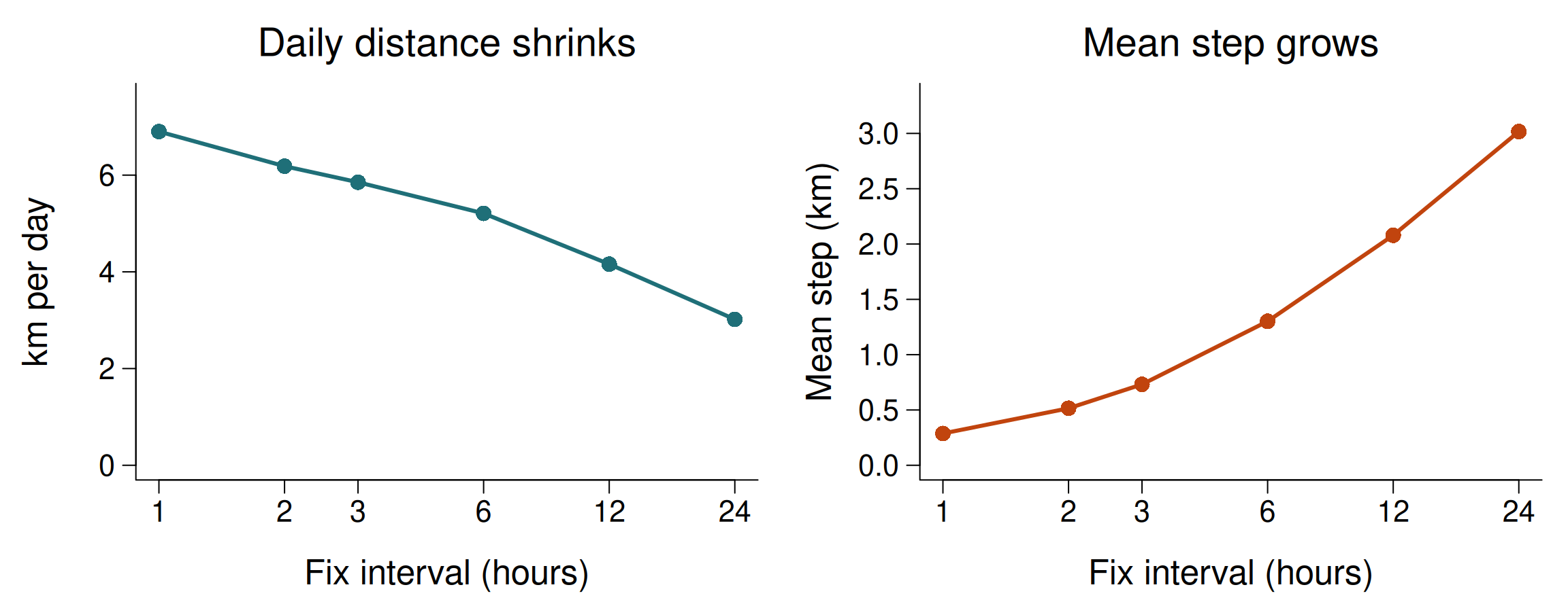
The same buffalo, Cilla, resampled to coarser and coarser intervals. Neither number is a property of the animal alone.

Straightness and sinuosity

Straightness index

\[\text{ST} = \frac{D}{L}\] Net displacement over path length, between 0 and 1.

Intuitive, but it depends on the length of the window you compute it over.

Sinuosity (Benhamou 2004)

Built from the step length and the concentration of turning angles.

Describes the local tortuosity of a random search path, and is far less sensitive to the window.

Use straightness for oriented movement (how directly did it get there?) and sinuosity for searching movement (how much does it wiggle?).

Fractal dimension

Measure path length with a “ruler” of length \(r\); on a fractal path \(L(r) \propto r^{1-D}\), so \(D\) comes from the slope of log L on log r
\(D = 1\): straight line; \(D \to 2\): a path that fills the plane
Appealing because it claims to be scale-free
The catch (Benhamou 2004; Turchin 1996): real animal paths are rarely fractal across more than a narrow range of scales, and \(D\) estimated from a correlated random walk varies with \(r\)

If \(D\) changes with the ruler, the path is not fractal — and the change itself tells you the scale at which the behaviour changes.

Net squared displacement (NSD)

\[\text{NSD}(t) = \lVert \mathbf{x}_t - \mathbf{x}_0 \rVert^2\]

The squared distance from the starting point. A remarkably effective diagnostic:

Sedentary — NSD rises then plateaus at a low value
Migratory — a sigmoid up, a plateau, a sigmoid back down
Dispersal — a single step up to a new plateau
Nomadic — rises roughly linearly, no plateau

Fitting these shapes as competing non-linear models (Bunnefeld et al. 2011) is a cheap and surprisingly effective way to classify movement strategies.

Four shapes

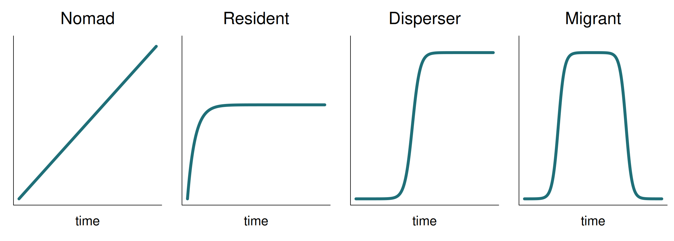
NSD against time for the four strategies of Bunnefeld et al. (2011).

Classifying strategies from NSD

Bunnefeld et al. (2011) fit competing non-linear models to each NSD curve and let the data choose:

Strategy	NSD shape	Model
Nomad	keeps rising	\(\beta t\)
Resident	rises, then plateaus	\(c\,(1 - e^{-kt})\)
Disperser	one sigmoid step	\(\delta / (1 + e^{(\theta - t)/\phi})\)
Migrant	up, plateau, back down	difference of two sigmoids

The fitted parameters are the biology: \(\sqrt{\delta}\) is the migration distance, \(\theta_1\) and \(\theta_2\) the departure and return dates. Never report the winning model without looking at them.

A real migrant: Leo

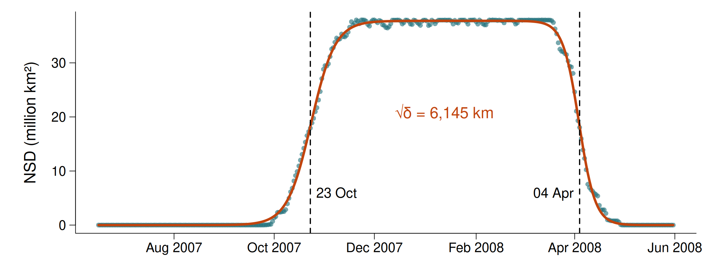
Daily NSD of the vulture Leo, June 2007 to May 2008, and the fitted migrant model. The parameters read as biology: a migration distance in thousands of kilometres, a departure date and a return date.

Quiz

You fit the four NSD models to a year of data for a savanna buffalo, and the migrant model wins by ΔAIC = 60. The fitted displacement is 12 km. What do you conclude?

The buffalo is a migrant
It shifted within its range; AIC picked the most flexible curve, and the parameters say it is not a migration
The resident model must have failed to converge
Buffalo cannot be classified with NSD

The double-sigmoid “migrant” curve is the most flexible of the four: it also fits an animal that drifts to one side of its home range for a few months and comes back. AIC rewards that fit — and with hundreds of autocorrelated daily points, AIC differences are grossly inflated.

The parameters settle it: 12 km is a home-range-scale shift. A real migrant such as Leo the vulture gives a displacement of thousands of kilometres. Read the parameters, not just the winner.

Quiz

Two studies report mean step length for the same population of roe deer. Study A reports 180 m, study B reports 640 m. Both are competent. What is the most likely explanation?

Study B’s collars had worse GPS accuracy
Study B sampled at a longer interval
Study B included migratory individuals
One of them made an arithmetic error

Step length scales with the sampling interval. An animal sampled hourly produces shorter steps than the same animal sampled every four hours, because the straight line between fixes cuts across all the wiggles in between.

This is why step length is not comparable across studies unless the interval matches, and why you must state the interval in every methods section.

It is also why Session 7’s step selection functions always compare an observed step with alternatives of exactly the same duration.

2 · First-passage time

How long to leave a circle?

Fauchald & Tveraa (2003): around each fix, draw a circle of radius \(r\) and measure the time the animal takes to leave it.

Where the animal searches intensively, first-passage time (FPT) is long; where it travels, FPT is short
Repeat for many radii and compute the variance of log FPT along the path
The radius at which that variance peaks is the spatial scale of area-restricted search

FPT turns “where does the animal slow down?” into a scale: how big are the patches it responds to?

First-passage time, drawn

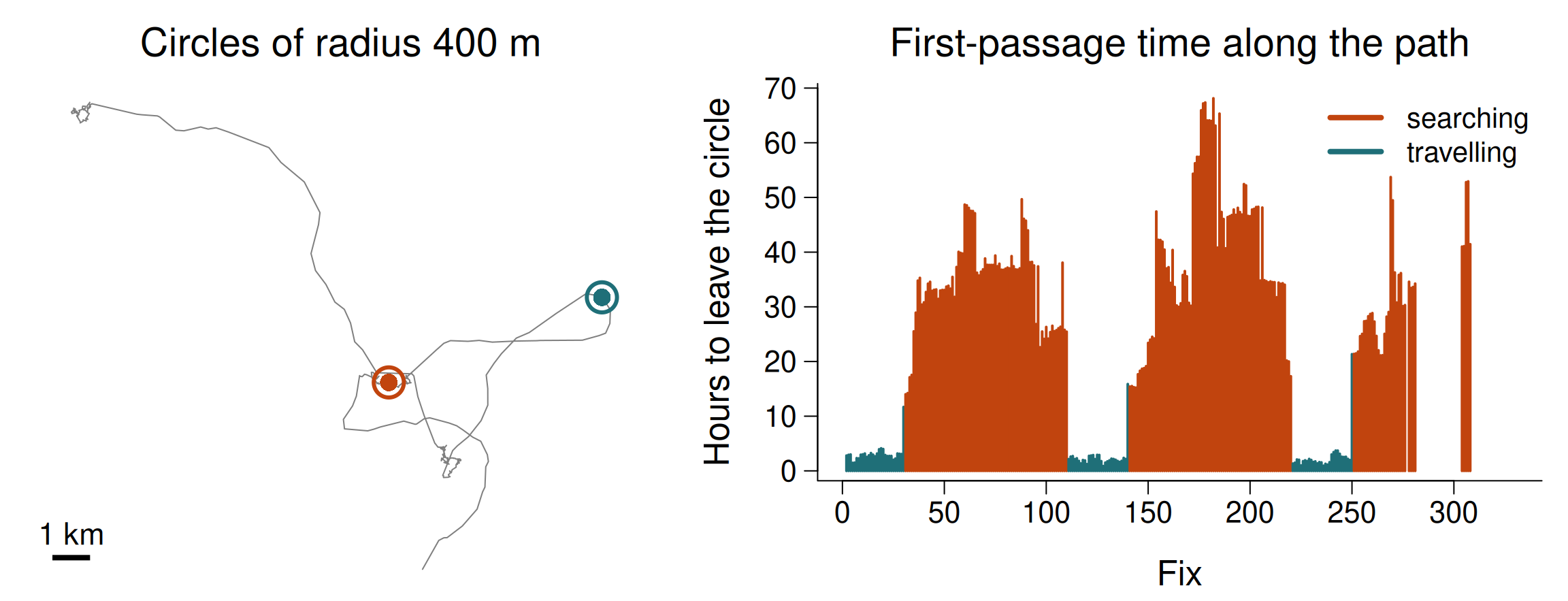
A simulated animal alternating travel and intensive search. Inside a patch it takes many hours to leave a 400 m circle; in transit, one or two.

Quiz

You compute var(log FPT) for radii from 25 m to 8 km for an hourly buffalo track. It is highest at 25 m, falls to a minimum at 1.5 km, then rises to a second peak near 4 km. Which peak is the scale of area-restricted search?

25 m — it is the highest
~4 km — the small-radius values are inflated by resting and GPS error
1.5 km — the minimum
Neither; FPT only works for seabirds

At radii comparable to GPS error and to the distance a resting animal shuffles, FPT is dominated by noise and by long bouts of doing nothing: its variance is high for reasons that have nothing to do with searching.

The meaningful signal is the peak at a scale well above the positional error — here about 4 km, the scale at which this buffalo concentrates its use. Always interpret FPT only for radii several times larger than your location error and typical resting movement.

3 · Behavioural modes

The problem

An animal is not doing one thing all day.

Resting, foraging, travelling, migrating — each with its own step-length and turning-angle signature
Pool them and every summary is a meaningless average: a “mean step length” that describes no actual behaviour
Leo’s six-year track contains residency and migration. A single home range spans two continents (Session 1)

Segment first, then analyse. Almost every method in this course assumes a homogeneous process. Segmentation is how you earn that assumption.

Encamped versus transit

The simplest useful classification has two modes:

Encamped

Short steps, frequent reversals, low net displacement.

Resting, ruminating, foraging within a patch.

Transit

Long steps, turning angles near zero, high net displacement.

Travelling between patches, to water, away from danger.

Finer schemes — resting / foraging / travelling — need either finer sampling or extra sensors (accelerometers). With hourly GPS, two or three modes is usually all the data can resolve.

Two questions, often confused

Change-point detection

“Where does the process change?”

Finds breakpoints in a time series. Output: a set of segments.

BCPA, segclust2d, penalised contrasts.

State classification

“Which of \(N\) recurring states is the animal in now?”

Assigns every step to a state, and states can recur.

HMM, EMbC, state-space models.

“Migration started on 14 September” is a change-point question. “Was this step foraging or travelling?” is a state question. Choose the tool that matches the question.

4 · Simple segmentation

The families

Approach	Idea	Notes
Thresholding	“Speed > 2 m/s = travelling”	Transparent; arbitrary; no uncertainty
First-passage time	Time to leave a circle of radius r	Good for finding scales of area-restricted search
BCPA	Change points in persistence velocity	Behavioural Change Point Analysis; needs a tuning choice
Clustering / EMbC	Cluster steps in (speed, turn) space	No time dependence — ignores that behaviour persists
HMM	Latent state chain + state-specific distributions	The standard. Uses time dependence
State-space models	HMM + explicit observation error	Handles messy data; slower, harder

Thresholds and expert rules

Speed threshold — “steps faster than \(v^*\) are travelling”. Transparent and reproducible
Expert rules — combine several: speed and turning angle and time of day, chosen from knowledge of the species
Both are defensible only when the metric is clearly bimodal — a histogram with an empty valley between modes
Without that valley, the threshold is an arbitrary decision dressed up as a result

An honest threshold, and a dishonest one

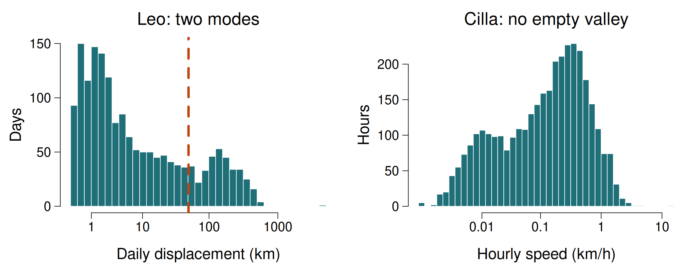
Left: Leo’s migration days (> 50 km, dashed) form a separate mode. Right: the buffalo’s speeds are a continuum with no gap; any cut-off is arbitrary.

Behavioural change-point analysis

BCPA (Gurarie et al. 2009) looks for places where the statistical properties of the movement change.

Works on a single variable, typically persistence velocity \(V\cos\theta\): fast and straight gives high values
Slides a window along the track; within each window finds the most likely break in mean, variance or autocorrelation
Collects breaks that recur across windows into change points
Works with irregular sampling, which is its great practical strength

BCPA tells you where the process changes. It does not tell you what the animal was doing, and it cannot know whether a change is behavioural or a change in your collar’s schedule.

BCPA on Cilla

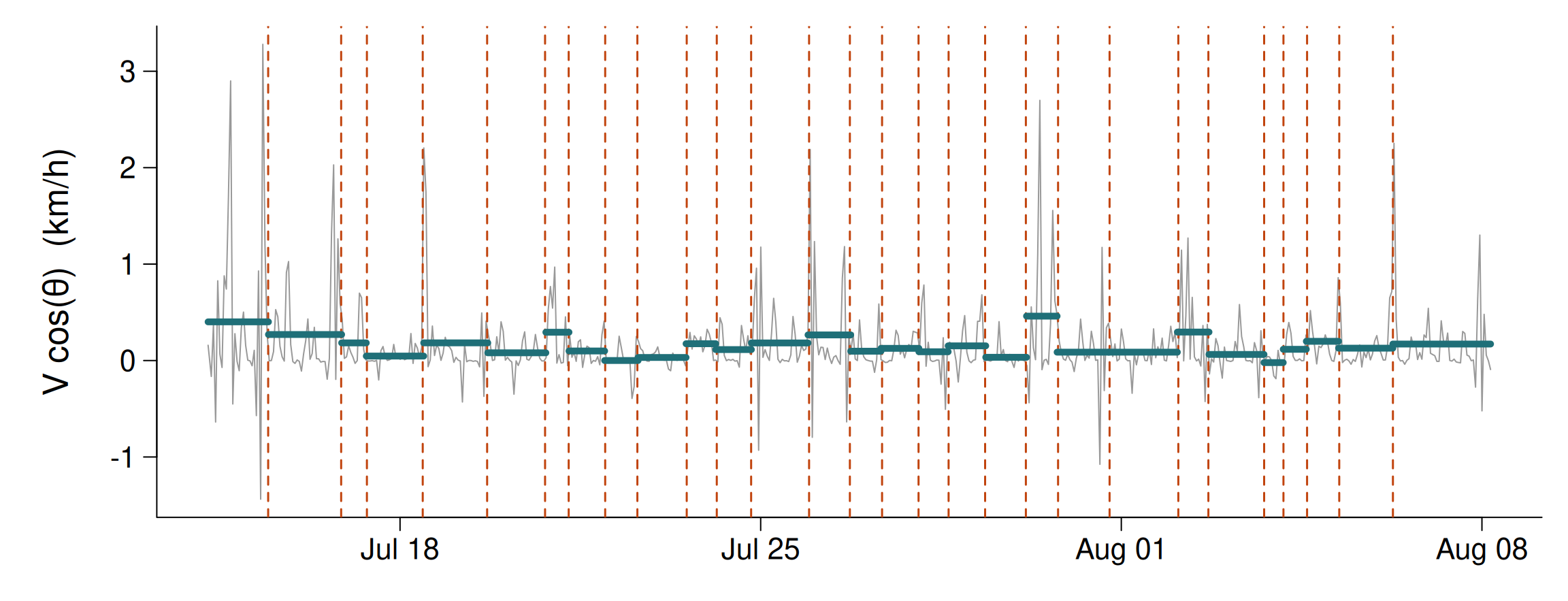
Persistence velocity over the first 25 days of hourly fixes (grey), the 28 change points BCPA finds with a 50-fix window (dashed), and the mean of each of the 29 phases (teal).

Quiz

BCPA on 25 days of hourly buffalo data, window of 50 fixes: 29 phases. Window of 30 fixes: 38. Same 50-fix window on the track resampled to 3-hourly: 19. How many behavioural phases did the buffalo go through?

29 — the default settings
19 — hourly data are too noisy
38 — more resolution finds more behaviour
The question has no single answer: phase counts depend on window size and fix rate

These are real results for the buffalo Cilla. The window size is an analyst’s tuning choice, and the fix rate sets what a “window of 50 fixes” means in time: 50 hours at hourly sampling, 150 hours at 3-hourly. Match the window in duration (17 fixes at 3-hourly ≈ 50 hours) and the 3-hourly count rises back to 29.

A phase count is a property of the analysis, not of the animal. What you can interpret biologically are the change points that persist across reasonable windows and fix rates — which is the robustness check you run in today’s practical.

Today’s practical

→ Session 4 practical

Net squared displacement with adehabitatLT — buffalo and vulture
Classify strategies: fit the four NSD models, then read the parameters
Straightness across scales
First-passage time and the scale of area-restricted search
A threshold that is honest (the vulture) and one that is not (the buffalo)
BCPA — and whether its answer survives a change of fix rate

Recap

Path descriptors — NSD, straightness, sinuosity, fractal dimension — all depend on the sampling interval and the window
NSD model classification is powerful; read the parameters, not just AIC
FPT finds the scale of area-restricted search — above the noise floor
Encamped versus transit is usually all hourly GPS can resolve
Thresholds are honest only across an empty valley; BCPA finds changes, not behaviours, and its answer depends on the fix rate

Before Session 5

Codling, Plank & Benhamou (2008), Random walk models in biology, J R Soc Interface 5:813 — sections 1–3
Make sure library(circular) loads

Questions?

giuliano.colosimo@uniroma2.it