Home ranges and space use

Session 6 — MCP → KDE → BBMM → AKDE

Giuliano Colosimo

University of Rome Tor Vergata

2026-10-06

Today

Internal state Motion capacity Navigation capacity External factors Movement path

A home range is what a path looks like when memory (navigation) and the distribution of resources (external factors) keep an animal in one place. Today: how to estimate it — and when it does not exist.

Where we are going

1. From territorial polygons to probabilistic utilisation distributions
2. MCP, and why it is still reported
3. Kernel density estimation, and its sensitivity to bandwidth
4. Autocorrelation: from nuisance (Brownian bridges) to information (AKDE)
5. When a home range is a valid concept: stationarity and the occupation timescale

Today’s real learning objective is the comparison: four estimators, one animal, four different answers — and a simulated animal whose true answer we know.

1 · What is a home range?

Burt’s definition

“That area traversed by the individual in its normal activities of food gathering, mating and caring for young.” — Burt (1943)

• Note what it excludes: exploratory forays, migration, dispersal
• Note what it does not say: nothing about probability, nothing about 95%
• Powell & Mitchell (2012): a home range is the part of its cognitive map an animal chooses to keep up to date — our estimators are crude proxies

From polygons to distributions

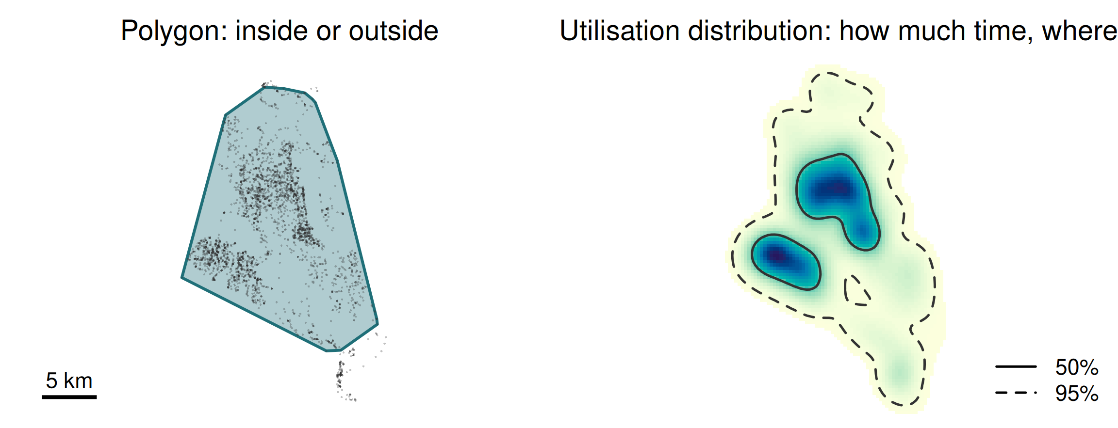
The same buffalo, Cilla. On the left every part of the area counts the same; on the right, core areas and rarely used edges are distinguished.

The UD is the object; “the home range” is a contour you draw on it. Say which contour, and which estimator produced the UD.

2 · Minimum convex polygon

MCP

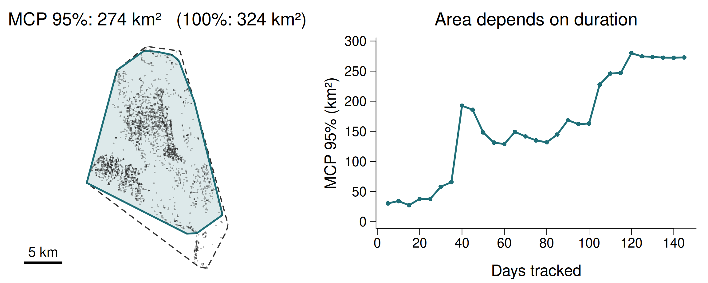
The smallest convex polygon containing \(x\)% of the fixes.

For

• Trivial to compute and explain
• Comparable with a century of literature
• No smoothing parameter to argue about

Against

• Convex — includes land never used
• Sensitive to outliers and sample size
• Area depends on how long you tracked
• No density information

Report it for comparability with old studies. Never as your only estimate.

MCP on a real buffalo

Left: the 95% MCP (solid) and 100% MCP (dashed) contain large stretches the animal hardly used. Right: the same estimate from the first 5, 10, 15… days.

3 · Kernel density estimation

KDE

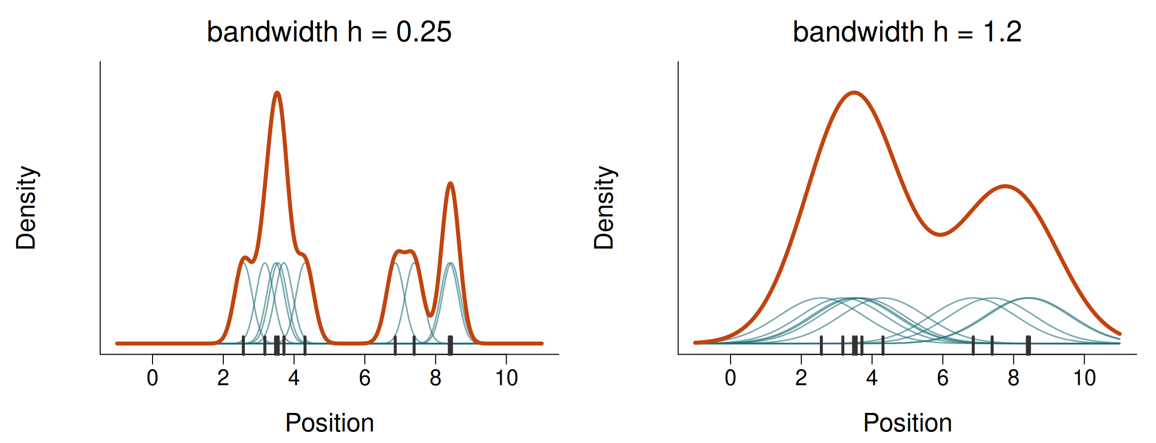
Put a small bump (kernel) on each fix and sum them into a utilisation distribution (Worton 1989).

• Gives a density: core areas, disjoint patches, used and unused parts
• The answer is dominated by the bandwidth \(h\)
  • \(h_\text{ref}\) — optimal if the UD were a single bivariate normal; usually over-smooths real, multi-modal ranges
  • \(h_\text{LSCV}\) — least-squares cross-validation; often under-smooths into fragments, and frequently fails to converge

How a kernel works

Ten fixes (ticks) in one dimension. Each gets a bump (thin lines); their sum (thick line) is the estimated UD. Same fixes, two bandwidths, two stories.

Same buffalo, two bandwidths

The buffalo Cilla, hourly fixes over 5 months, 95% contours:

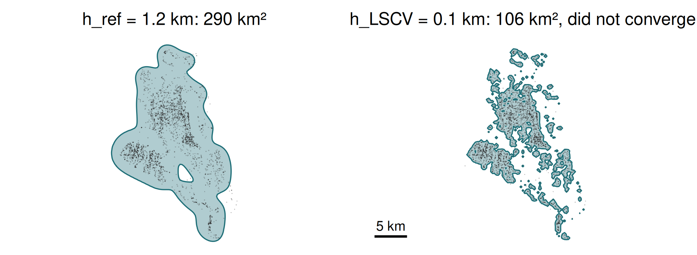
A factor of three from one analyst’s choice. Report the bandwidth selector — and check whether LSCV actually converged. adehabitatHR warns you; papers rarely do.

Quiz

You compute a 95% KDE with LSCV and get a range three times smaller than with \(h_\text{ref}\), made of dozens of small islands. kernelUD() printed “the algorithm did not converge”. What do you report?

• The LSCV result — it is data-driven and \(h_\text{ref}\) is known to over-smooth
• The average of the two
• That the KDE area is not well determined by these data, and prefer an estimator that accounts for autocorrelation
• The \(h_\text{ref}\) result, because it converged

LSCV fails in a characteristic way on GPS data: with many autocorrelated fixes it chooses a tiny bandwidth that treats every cluster of consecutive fixes as a separate hotspot. A non-converged bandwidth is not a result.

\(h_\text{ref}\) “converges” only because it is a formula — it assumes a unimodal range and has no way to be wrong in public. Neither is trustworthy here. The disagreement itself is the finding: these data do not pin down a KDE area, which points to the autocorrelation-aware methods on the next slides.

4 · Autocorrelation

The problem classical KDE has with GPS

Classical KDE assumes fixes are independent draws from the UD.

Hourly GPS fixes are nothing of the sort — the animal was 300 m away an hour ago and will be 300 m away in an hour.

• The effective sample size is far smaller than \(n\)
• The UD comes out too narrow — the range is under-estimated
• Collecting more fixes at a higher rate makes it worse, not better

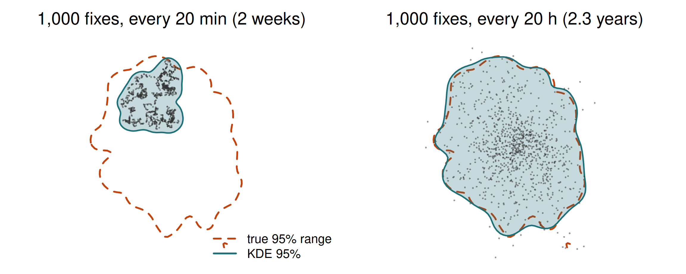
This is why area estimates from 1990s VHF studies (a few dozen fixes, days apart) and modern GPS studies (thousands, an hour apart) are not comparable.

Same number of fixes, different information

The central-place animal from Session 5, whose true range (dashed) we know. Two weeks of dense fixes describe two weeks of the animal, not its range.

Brownian bridges: use the path

Horne et al. (2007): between two consecutive fixes the animal was somewhere on a random bridge connecting them.

• The uncertainty of the bridge grows with the time gap and shrinks near each fix, scaled by a mobility parameter estimated from the data
• Uses the order of the fixes, not just their positions
• Handles irregular sampling naturally
• Answers a specific question: where was the animal during the tracking period? — its occurrence distribution

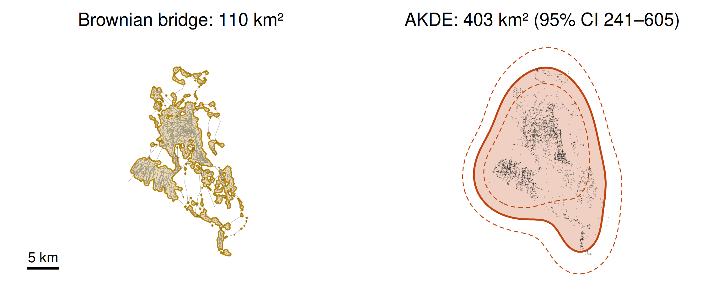
A Brownian bridge maps where the animal went, not where it could go. It shrinks around the observed path, so it is usually the smallest of the estimates — correctly so, for the question it answers.

Autocorrelation is information

Fleming et al. (2015): stop treating autocorrelation as a nuisance.

1. Fit a continuous-time movement model to the track (ctmm)
2. The model tells you how long the animal takes to cross its range — the range-crossing time \(\tau_\text{position}\)
3. From that, the effective sample size: roughly how many times the animal crossed its range during tracking
4. Weight the kernel accordingly: AKDE

AKDE estimates the range distribution — where the animal would be found in the long run — and gives it a confidence interval. If you track for three range-crossing times, you effectively have three observations, however many fixes you collected.

Where it went, where it lives

Cilla again, on the same scale. The bridge hugs the path she travelled; AKDE estimates the range she would use given time, with its confidence interval (dashed).

The variogram

The semi-variance as a function of time lag: how far apart, on average, two positions \(\Delta t\) apart are.

• Rises at short lags as the animal moves away
• Levels off at an asymptote if the animal is range-resident: beyond the range-crossing time, positions are as far apart as they will ever be
• Keeps rising if the animal is not range-resident — drifting, dispersing, nomadic
• Proportional to the mean squared displacement of Session 5: the same curve, rescaled

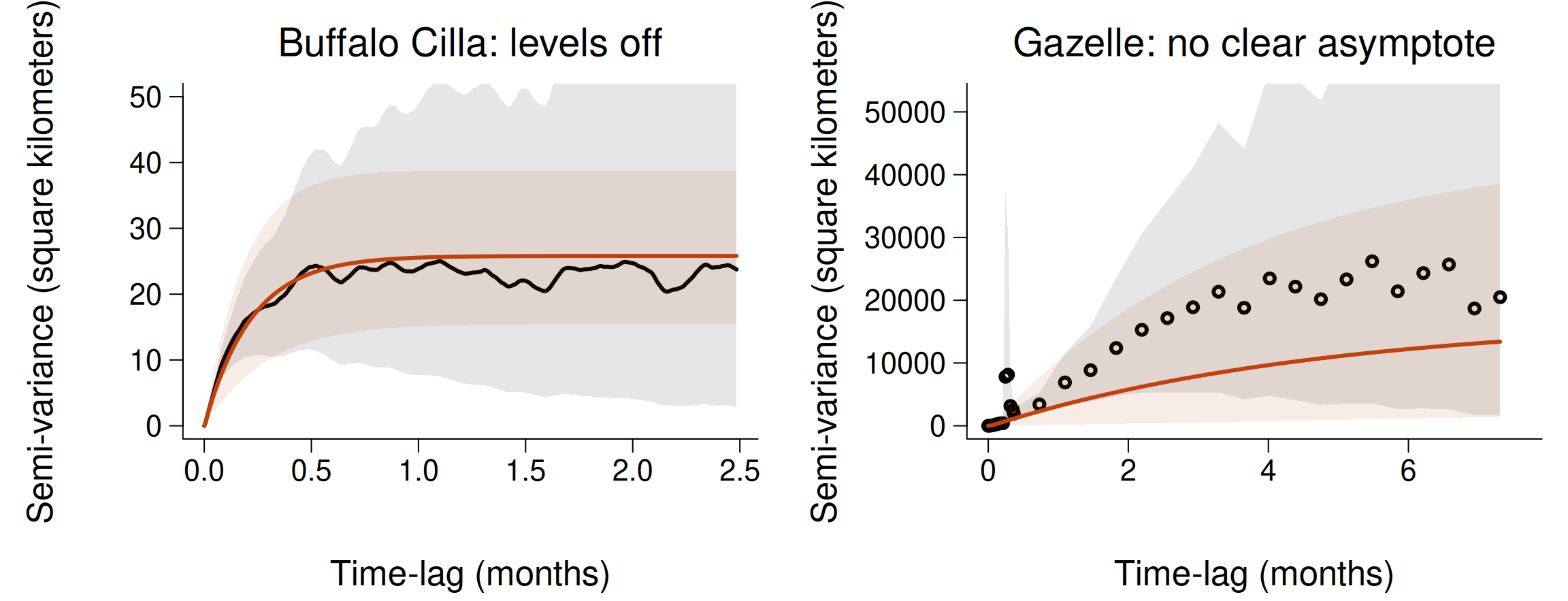
Look at the variogram before estimating any home range. No asymptote, no home range.

Two variograms

Black: data. Red: fitted model. Cilla’s range-crossing time is ~6 days, so her 3,500 fixes are worth ~19 independent ones. The gazelle’s is ~5 months: two or three crossings in a year.

Quiz

A Mongolian gazelle tracked for a year has an estimated range-crossing time of ~5 months (95% CI: 1 to 27 months), and its variogram shows no clear asymptote. What should you conclude?

• Its home range is about 300,000 km², as AKDE reports
• You need more fixes per day
• The animal is not demonstrably range-resident at the scale of the study; a home range is not a meaningful summary
• Switch to MCP, which does not need an asymptote

These are the real ctmm results for a gazelle in the package’s example data. A range-crossing time whose upper bound exceeds the whole tracking period means the animal crossed its “range” perhaps two or three times, or perhaps never: the effective sample size is tiny and the area’s confidence interval spans an order of magnitude.

More fixes per day do not help: the constraint is duration, not frequency. And switching to MCP hides the problem without solving it. Mongolian gazelles are nomadic; for them, a home range may simply be the wrong concept.

5 · When is a home range valid?

Stationarity and the occupation timescale

• Every estimator assumes the UD is stationary over the tracking period: the animal’s space use is not systematically changing
• Seasonal shifts, dispersal and migration all violate it — segment first (Session 4) and estimate one range per stationary period
• The track must be much longer than the range-crossing time, or the animal has not yet shown you its range
• In Session 5, a buffalo tracked for 36 days was indistinguishable from a random walker; one tracked for 157 days was clearly confined

“Must the time series be stationary?” Yes — over the timescale you summarise. A home range is always a home range for a stated period.

Choosing an estimator

	Answers	Use when	Watch out for
MCP	outer boundary	comparing to old literature	convexity, outliers, sample size
KDE	density of fixes	many roughly independent fixes	bandwidth; autocorrelation
BBMM	where it went	the path matters; irregular data	not a long-run range
AKDE	where it lives	modern GPS data: the default	needs range residency

And before any of them: should you be estimating a home range at all? Check the variogram, and check that the track is stationary.

Quiz

For one buffalo you get 95% areas of: MCP 274 km², KDE (\(h_\text{ref}\)) 290 km², Brownian bridge 110 km², AKDE 400 km². Which statement is correct?

• AKDE is wrong because it disagrees with the others
• The Brownian bridge is wrong because it is the smallest
• BBMM and AKDE answer different questions — where it went versus where it lives
• The average, 269 km², is the best estimate

These are the real values for the buffalo Cilla. The Brownian bridge estimates the occurrence distribution — the area around the path actually travelled during tracking — so it hugs the path. AKDE estimates the range distribution — where the animal would be found in the long run — and inflates the area to account for the parts of the range the animal would visit given more time.

Averaging estimates of different quantities produces a number that answers no question. Choose the estimator from the question, and state the question.

Today’s practical

→ Session 6 practical

1. MCP, KDE (\(h_\text{ref}\) and LSCV), Brownian bridge and AKDE for one buffalo
2. Map all four; write one paragraph on why they differ
3. Variograms: a resident buffalo versus a nomadic gazelle
4. Ground truth: estimate the home range of the simulated animal from Session 5, whose true range we know — and see how each estimator fails

Recap

• The UD is the object; a home range is a contour on it
• MCP for comparability only; KDE depends on bandwidth and ignores autocorrelation
• Brownian bridges map occurrence; AKDE estimates the range with a CI
• Autocorrelation is information: effective sample size = range crossings
• Check the variogram and stationarity first

Before Session 7

• Fieberg et al. (2021), J Anim Ecol 90:1027 — the “how-to” guide to habitat-selection parameters. The most useful paper of the course
• Fortin et al. (2005), Ecology 86:1320 — the first step selection function

Questions?

giuliano.colosimo@uniroma2.it