Habitat selection on the move

Session 7 — Resource selection and step selection functions

Giuliano Colosimo

University of Rome Tor Vergata

2026-10-06

Today

Internal state Motion capacity Navigation capacity External factors Movement path

Where does an animal go, given what is available to it — and how does the environment change the way it moves? Today separates those two questions and then fits them together.

Where we are going

Use versus availability, and the orders of selection
Designs: used–available (RSF), used–unused (RSPF), matched steps (SSF)
The SSF as conditional logistic regression (Fortin et al. 2005)
Integrated SSA: movement and selection estimated together (Avgar et al. 2016)
From coefficients back to a predictive movement model

1 · Use versus availability

Selection is a comparison

An animal selects a resource when it uses it disproportionately to its availability.

Use alone tells you nothing. A wolf in a landscape that is 95% forest will be found mostly in forest whether or not it prefers forest
So every selection analysis needs two samples:
- Used — where the animal was
- Available — where it could have been

The second sample is not data. You construct it, and the construction encodes a hypothesis. Most disagreements about habitat selection results are disagreements about availability.

Used and available, for one fisher

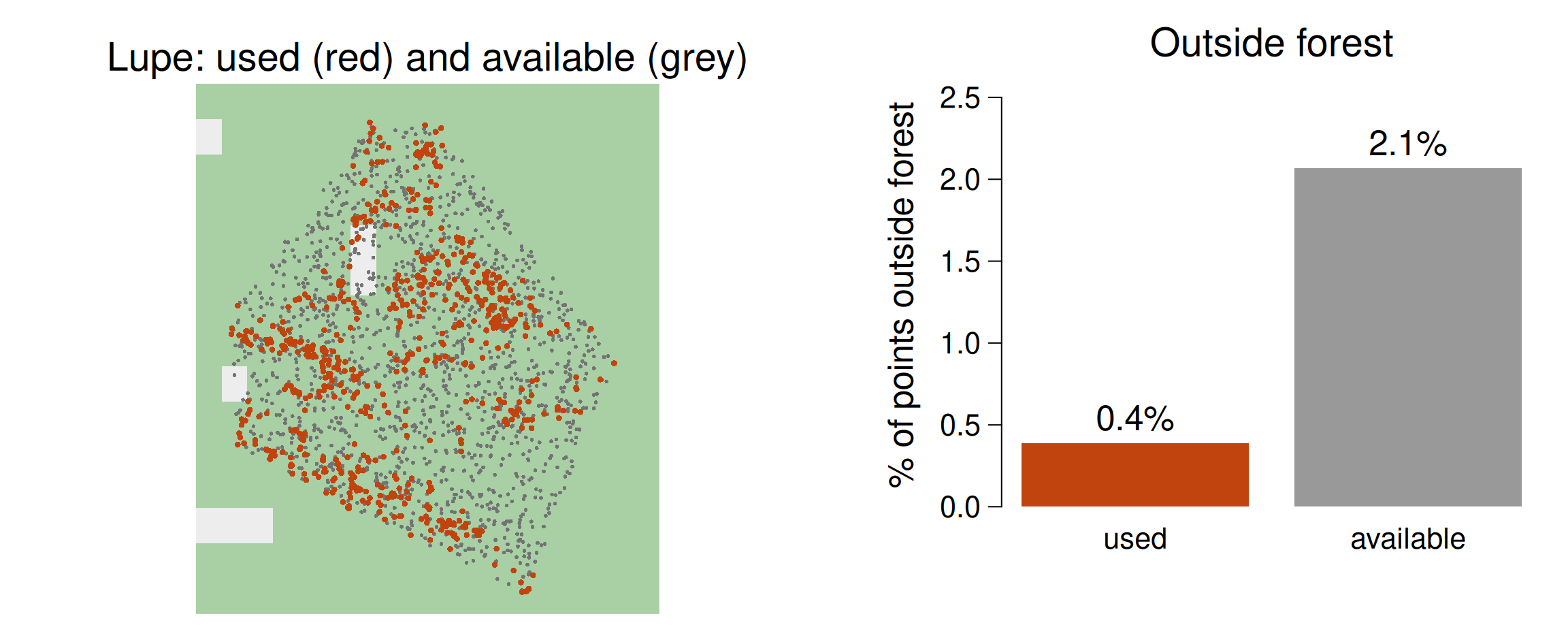
Green: forest. Almost every fix is in forest — but so is almost everything available. The signal is in the comparison: outside forest, Lupe turns up 5 times less often than availability predicts.

Johnson’s four orders (1980)

Order	Question	Available =
1st	Where is the species’ range?	The planet
2nd	Where does this individual put its home range?	The study area / population range
3rd	Where within its home range does it go?	The home range
4th	Which items does it take at a site?	Items at the site

The same animal can show opposite results at different orders. A deer may place its home range in forest (2nd order) yet prefer clearings within it (3rd order). Always state your order — it is the definition of “available”.

Quiz

Two studies of the same wolf population reach opposite conclusions about selection for roads. Study A used available points drawn from the whole national park; study B drew them from within each wolf’s home range. Who is right?

Study A — a larger availability domain is more objective
Study B — home ranges are the only biologically meaningful domain
Both, and they answer different questions
Neither; the analysis is invalid without known absences

Study A asks a second-order question: given the whole park, do wolves put their home ranges in areas with more or fewer roads? Study B asks a third-order question: within the home range a wolf has already chosen, does it approach or avoid roads?

These routinely give opposite answers, and the pattern is common and interpretable: wolves may settle in road-poor parts of the park (avoidance at 2nd order) while using road verges and tracks as travel routes once there (selection at 3rd order).

Neither study is wrong. Both are incomplete if they do not state the order and the availability domain — which is why that belongs in the abstract, not buried in the methods.

2 · Three designs

Used–available, used–unused, matched

Design	Compares	Estimates	Model
Used–available (RSF)	fixes vs random points in a domain	relative selection	logistic, weighted
Used–unused (RSPF)	sites used vs sites known to be unused	absolute probability of use	logistic
Matched steps (SSF)	each step vs steps available from the same point	relative selection, conditional on movement	conditional logistic

Absolute probabilities need genuine absences — sites surveyed and known to be unused (Lele & Keim 2006 discuss when an RSPF is estimable). Telemetry almost never provides them, which is why almost every tracking study fits an RSF or an SSF and reports relative selection.

Availability, three ways

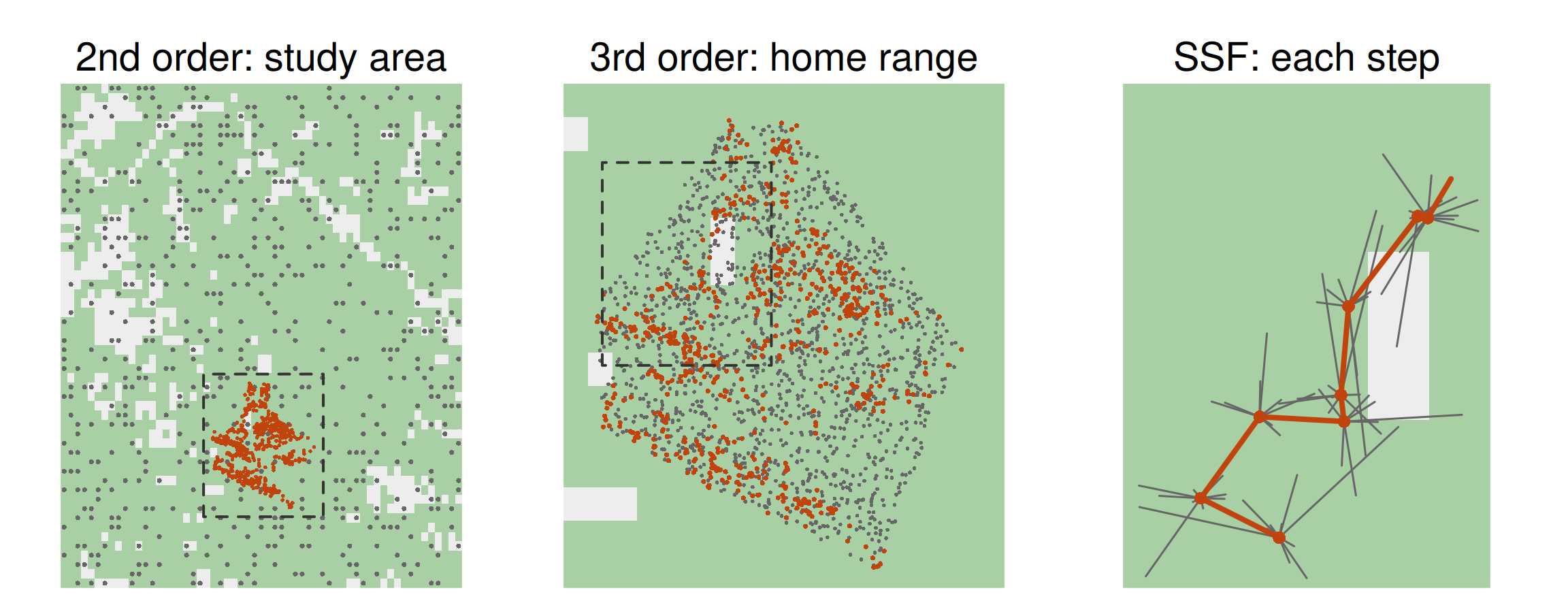
The same fisher (red). Each panel zooms into the dashed box of the previous one: the study area, the home range, and eight steps with their control steps (grey).

The RSF

\[w(\mathbf{x}) = \exp(\beta_1 x_1 + \beta_2 x_2 + \cdots + \beta_k x_k)\]

\(w(\mathbf{x})\) is the relative probability of use, proportional to the true probability by an unknown constant.

Fitted with logistic regression on used (1) vs available (0) points
There is no intercept you can interpret — it absorbs the arbitrary number of available points you drew
Only relative statements are licensed: “twice as likely as”, never “40% probability of use”

Used–available is not case–control

“Available” points are not known absences. The animal may well have used them; you just did not observe it
Formally, the used–available design fits an inhomogeneous Poisson point process, and logistic regression is a computational device for it
This is why the infinitely weighted logistic regression trick works: give available points a huge weight and the logistic coefficients converge to the correct point-process coefficients

d$w <- ifelse(d$case_, 1, 5000)
glm(case_ ~ elevation + grassland, data = d,
    family = binomial(), weights = d$w)

Quiz

Your RSF gives \(\hat\beta = 0.69\) for a standardised NDVI covariate. What can you correctly say?

There is a 69% probability the animal uses high-NDVI areas
A one-SD increase in NDVI roughly doubles the relative probability of use
NDVI explains 69% of the variation in use
The animal uses high-NDVI areas 69% of the time

RSF coefficients are on the log scale, so the effect is multiplicative: \(e^{0.69} \approx 2\). A one-standard-deviation increase in NDVI doubles the relative probability of use, holding the other covariates fixed.

“Relative” is doing essential work in that sentence. The RSF is proportional to the probability of use by an unknown constant — the intercept depends entirely on how many available points you happened to draw — so absolute probabilities are not available to you.

Standardising covariates before fitting is what makes “one SD” meaningful and lets you compare effect sizes across covariates measured in different units.

Three decisions

The domain. Study area? MCP? KDE? Buffer around the track? This is your choice of Johnson order.
How many points. Too few and the estimates are noisy; the coefficients should stabilise as you add more. Check that they do.
How they are distributed. Uniform random is the default. But should inaccessible areas (open water, cliffs, the other side of a motorway) be “available” at all?

Changing the availability domain can reverse the sign of a coefficient. This is not a flaw in the method — it is the method working. Different domains ask different questions.

Do the coefficients stabilise?

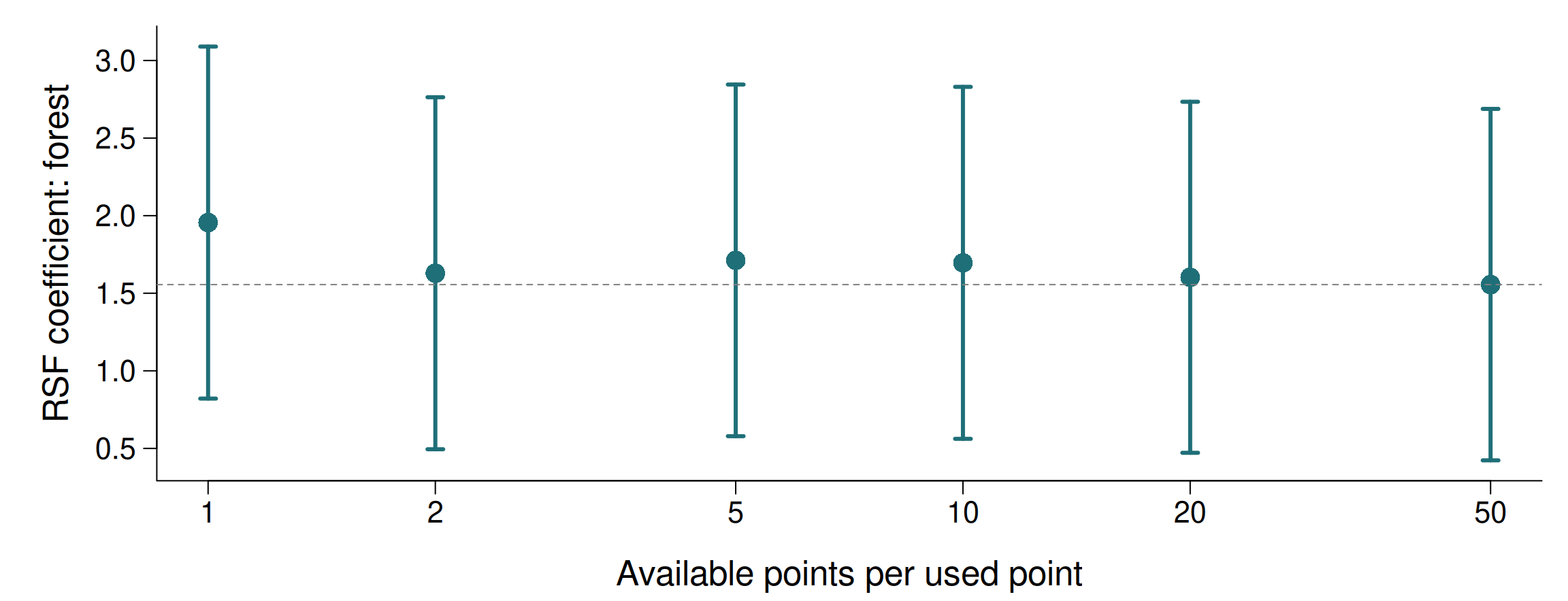
Lupe’s forest coefficient and 95% CI, refitted with more and more available points. The estimate settles by about ten per fix; the interval hardly narrows, because the information is in the 774 used fixes.

3 · Step selection functions

An animal cannot be anywhere

An RSF treats every point in the home range as equally available at every moment
But a buffalo at 08:00 cannot be 20 km away at 09:00. It can reach perhaps a kilometre
So most of the “available” set was never a real alternative
Availability is local, and it moves with the animal

A step selection function fixes this by defining availability from the animal’s own movement capacity: from where it was, where could it plausibly have gone?

The design

For each observed step:

Take the starting point \(\mathbf{x}_{t}\)
Draw \(k\) control steps from the animal’s own distributions of step length and turning angle
That gives one stratum: 1 used step + \(k\) available steps, all from the same starting point at the same time
Compare them with conditional logistic regression

Because the comparison is within a stratum, everything constant at that moment — time of day, season, the animal’s internal state, its identity — cancels out. That is a remarkably clean piece of control.

One stratum

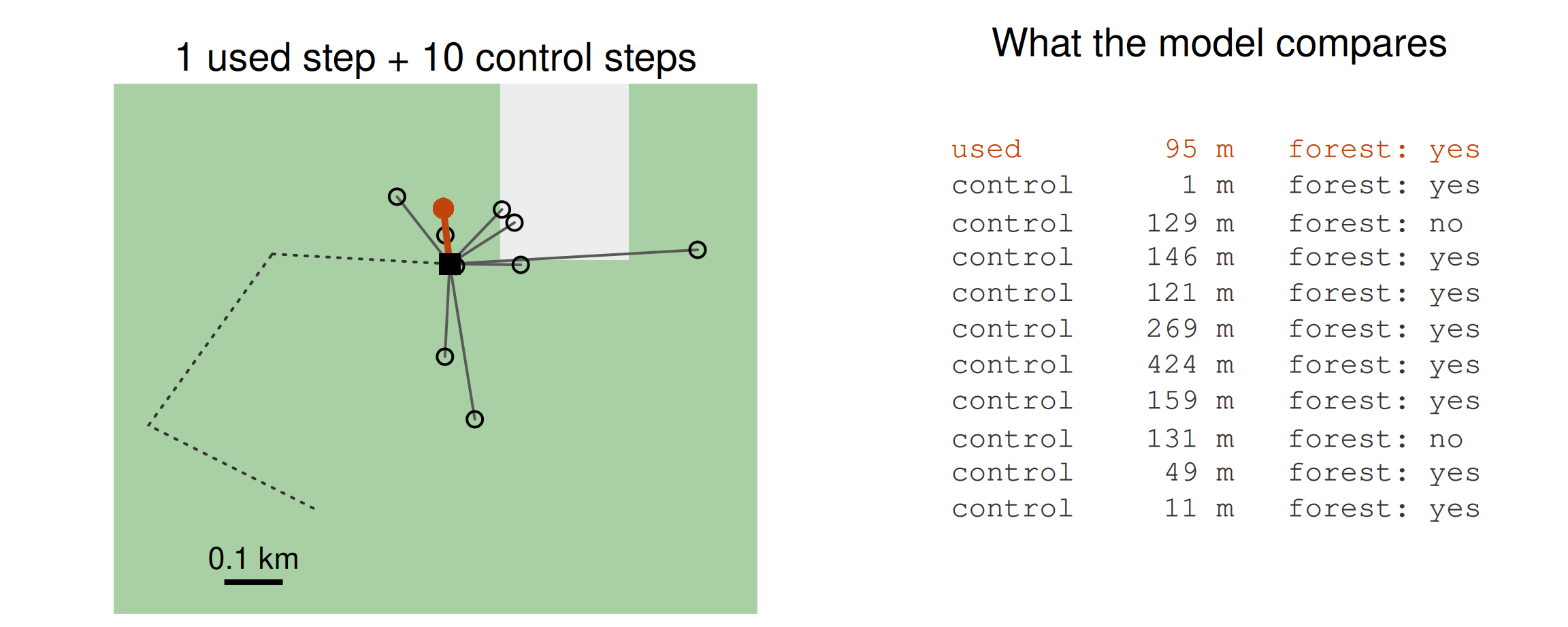
Square: where the fisher was. Dotted: the steps that brought it there. The model asks only how the used step differs from its own controls.

Conditional logistic regression

\[ P(\text{step } j \text{ chosen}) = \frac{\exp(\boldsymbol{\beta}^{\top}\mathbf{x}_j)} {\sum_{i \in \text{stratum}} \exp(\boldsymbol{\beta}^{\top}\mathbf{x}_i)} \]

Identical machinery to a Cox proportional hazards model — which is why survival::clogit() and amt::fit_issf() both go through coxph()
Each stratum contributes only the contrast between the used step and its controls
No intercept. Again, only relative statements

fit_issf(case_ ~ elevation_end + sl_ + log(sl_) +
                 strata(step_id_),
         data = d)

Fortin et al. (2005)

The paper that made SSFs standard: elk in Yellowstone after wolves returned.

Each observed step compared with control steps drawn from the elk’s own step-length and turning-angle distributions
Elk avoided aspen stands in areas with high wolf density
The effect changed where elk browsed, and so which aspen could regenerate — a behavioural route to a trophic cascade

The SSF made it possible to ask how predators change fine-scale movement decisions, not just where prey live.

Quiz

Why does a step selection function include strata(step_id_)?

To account for repeated measures on the same animal
Because each used step is compared only with the control steps drawn from its own starting point and time
To weight the available points correctly
It is optional; it only speeds up fitting

The stratum is the design. Each observed step is matched to the controls generated from the same location at the same moment, and the likelihood only ever compares within that matched set.

This is what makes availability local and time-specific — and it means anything constant within the stratum (hour of day, season, weather, the animal’s identity and internal state) is automatically controlled for, without you having to model it.

Individual-level repeated measures are a separate issue, handled by fitting per animal or by a mixed conditional model (Muff et al. 2020). Dropping strata() does not merely change the standard errors — it fits an entirely different, and wrong, model.

4 · Integrated step selection

The circularity problem

To generate control steps you need the animal’s step-length and turning-angle distributions. But those distributions are themselves affected by habitat — an animal moves slowly in good habitat and fast through bad.

Estimate them from the raw data, and they are already contaminated by selection
Use them to define availability, and you bake the contamination in
The estimated selection coefficients are then biased

Integrated step selection analysis (Avgar et al. 2016) solves this by estimating the movement kernel and the selection coefficients simultaneously, from the same model.

How iSSA does it

Include the movement variables as covariates in the conditional model:

sl_ and log(sl_) — together these correct the gamma step-length distribution used to generate the controls
cos(ta_) — corrects the von Mises turning-angle concentration
The fitted coefficients on these terms tell you how the realised movement kernel differs from the tentative one you sampled from

fit_issf(case_ ~ elevation_end + grassland_end +
                 sl_ + log(sl_) + cos(ta_) +
                 strata(step_id_), data = d)

Reading the movement coefficients

If controls were drawn from a gamma with shape \(k\) and scale \(\theta\):

Term	Effect on the realised kernel
\(\beta_{\log(sl)}\)	adjusts shape: \(k_{\text{real}} = k + \beta_{\log(sl)}\)
\(\beta_{sl}\)	adjusts scale: \(1/\theta_{\text{real}} = 1/\theta - \beta_{sl}\)
\(\beta_{\cos(ta)}\)	adjusts concentration: \(\kappa_{\text{real}} = \kappa + \beta_{\cos(ta)}\)

A positive \(\beta_{\cos(ta)}\) means the animal moves more directionally than your tentative distribution assumed. amt::update_gamma() and update_vonmises() do this arithmetic for you — use them rather than doing it by hand.

Tentative and realised kernels

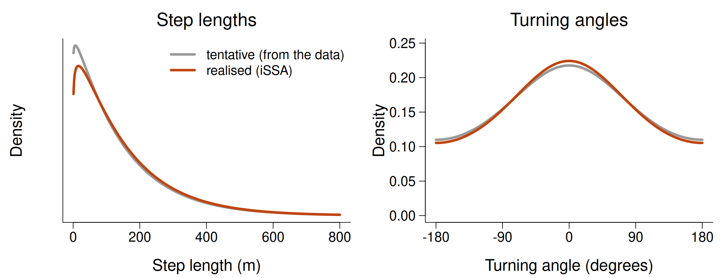
Grey: the distributions Lupe’s control steps were drawn from. Red: the movement kernel after the iSSA correction. For this fisher the correction is small (mean step 147 → 154 m); it is large when habitat strongly shapes how far an animal moves.

Interactions: where it gets interesting

The real power is asking whether movement depends on habitat:

case_ ~ grassland_end +
        sl_ + log(sl_) + cos(ta_) +
        sl_:grassland_start +        # faster in grassland?
        cos(ta_):grassland_start +   # straighter?
        strata(step_id_)

_start covariates modify the movement kernel — how the animal moves from that habitat
_end covariates capture selection — which habitat it moves into
Mixing them up is the single most common error in iSSA papers

Quiz

In an iSSA you find a positive coefficient on sl_:forest_start. What does it mean?

The animal selects forest
The animal takes longer steps when starting from forest — it moves through forest faster
Forest patches are larger than other patches
Steps ending in forest are longer

An interaction with sl_ modifies the movement kernel, not the selection term, and _start means the covariate is measured at the step’s origin. So this says: given that the animal is in forest, its steps are longer.

Ecologically that usually means the animal is transiting, not using, the forest — it crosses quickly rather than lingering.

Note how this can coexist with positive selection for forest (forest_end > 0): an animal may head into forest and then move through it rapidly. Separating “where does it go” from “how does it move once there” is exactly what iSSA buys you, and it is invisible to an RSF.

5 · The iSSF payoff

From coefficients back to movement

An iSSA gives you two things at once:

a movement kernel — how far and how straight the animal moves, and how that depends on where it is
a selection function — which destinations it prefers

Multiply them and you have the animal’s redistribution kernel: the probability of being at each place one step from now. Iterate it, and you simulate new tracks — in the current landscape, or in one you are planning to change.

That is the bridge to mechanistic models: a fitted iSSA is a generative model of movement, like the random walks of Session 5, but with the environment built in.

A redistribution kernel, built

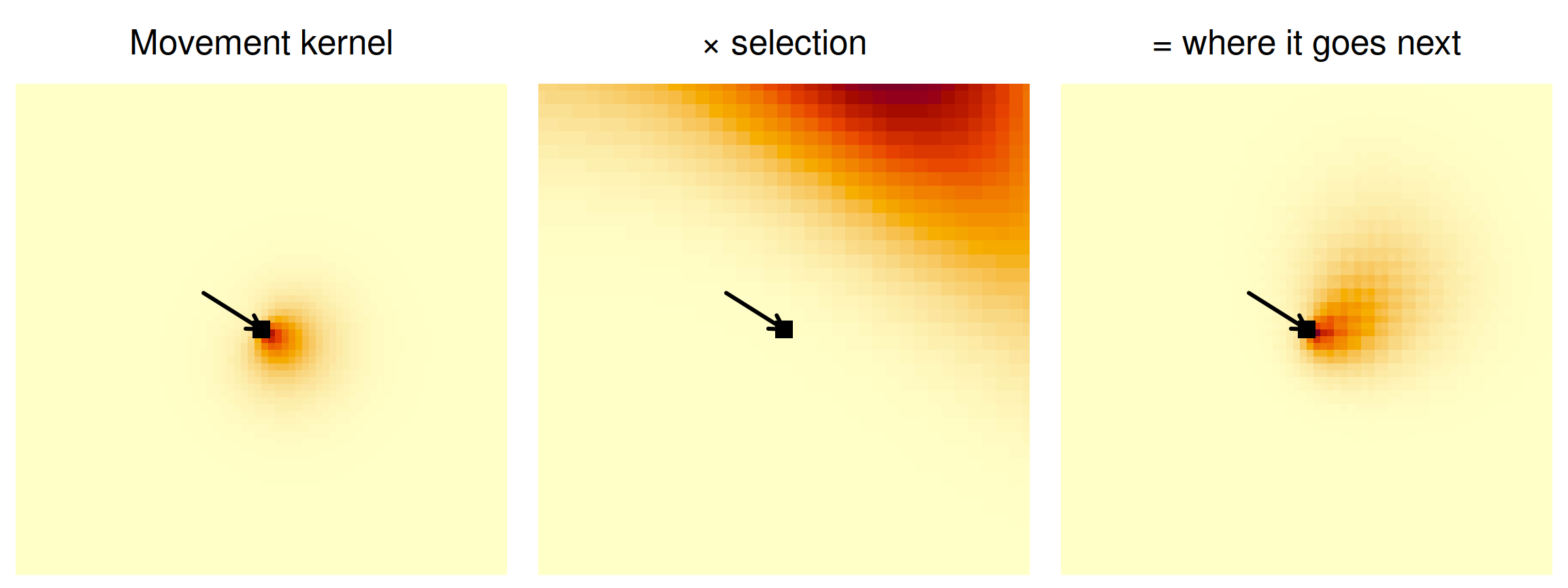
The simulated animal of today’s practical (β = 1.5) in a 1.8 km window. Square: where it is; arrow: its last step. Movement says how far and which way; selection tilts the kernel towards better habitat.

Relative selection strength

The natural effect size for an SSF (Avgar et al. 2017; Fieberg et al. 2021):

\[\text{RSS}(x_1, x_2) = \exp\big(\beta\,(x_1 - x_2)\big)\]

“How many times more likely is the animal to take a step ending at \(x_1\) rather than \(x_2\), given both were equally reachable?”
For a binary habitat, RSS = \(e^{\beta}\)
For a continuous covariate, RSS depends on the difference you pick — report it for a biologically meaningful one

6 · Doing it well

Practical decisions

How many control steps? 10 is a common default; check that coefficients stabilise as you increase it, exactly as for RSF availability
Sampling interval. All steps in the analysis must share one duration. Resample first (Session 3)
Where to measure covariates. At the end point, along the step, or averaged over it? Measuring along the step is more defensible for barriers such as roads and rivers
Zero-length steps break the gamma distribution — amt warns and replaces them

Multiple animals, again

Two-stage: fit each animal, then summarise the coefficients. Simple, transparent, and adequate for small samples
Mixed conditional models: Muff et al. (2020) show how to fit these in glmmTMB with random slopes and a fixed large variance on the stratum intercepts
A random intercept alone is not enough — it does not let individuals differ in selection, which is usually the biology you care about

Validation

Used–habitat calibration plots (Fieberg et al. 2018)
Withhold whole individuals, or whole time blocks — never random steps, because autocorrelation leaks the answer into the test set
Simulate from the fitted model and compare the simulated space use with the observed. If your model cannot regenerate something resembling the real track, it has not captured the process

amt::simulate_path(...)   # redistribution kernel from the fitted iSSA

Quiz

You fit an iSSA with 10 control steps per stratum, then refit with 100. The coefficients barely move but all the standard errors halve. What do you report?

The 100-control model — smaller standard errors are better
Either set of coefficients, but do not treat the smaller SEs as stronger evidence about the animal
The 10-control model, because 100 is overfitting
Neither; the discrepancy means the model is misspecified

Stable coefficients are exactly what you want to see — it means 10 controls already characterised availability well, and that is the check worth reporting.

The shrinking standard errors are the same trap as with RSF availability. Control steps describe what was available, which you can sample as finely as you like. More of them sharpen your description of availability; they do not constitute additional observations of the animal’s choices. Your real sample size is the number of steps — and, for population inference, the number of animals.

Report the effect sizes, state how many controls you used, and show that the estimates were stable with respect to that choice.

RSF or SSF?

	RSF	SSF / iSSA
Availability	Whole domain, fixed	Local, moves with the animal
Order	Usually 2nd or 3rd	Effectively 3rd, step-scale
Needs regular sampling	No	Yes
Models movement	No	Yes
Time-varying covariates	Awkward	Natural
Best for	Broad-scale range placement	Fine-scale decisions, corridors, barriers

If your data are regularly sampled and you care about how the animal moves through the landscape, use iSSA. If your sampling is sparse or irregular, and your question is about broad-scale range placement, an RSF is the honest choice.

Today’s practical

→ Session 7 practical

An RSF for a fisher, with used and available points
The same fisher as an SSF: random steps, extract_covariates(), fit_issf()
Relative selection strength, and the realised movement kernel
Habitat-mediated movement: interactions with _start covariates
Ground truth: recover a known selection coefficient from a simulated animal

Recap

Selection = use relative to availability; state the order and the domain
RSF: used vs available; RSPF needs real absences; SSF: each step vs its own alternatives
strata(step_id_) is the design, not a detail
iSSA estimates movement and selection together; _end covariates select, _start covariates modify movement
A fitted iSSA is a generative model: it can simulate

Before Session 8

McClintock et al. (2020), Uncovering ecological state dynamics with hidden Markov models, Ecology Letters 23:1878 — sections 1–3
Make sure library(momentuHMM) loads, and prepare a 3–5 minute mini-project pitch

Questions?

giuliano.colosimo@uniroma2.it