Hidden Markov models and synthesis

Session 8 — Behavioural states, the research frontier, mini-project pitches

Giuliano Colosimo

University of Rome Tor Vergata

2026-10-06

Today

Internal state Motion capacity Navigation capacity External factors Movement path

A hidden Markov model is the most direct attempt in the course to infer the internal state from the path — and to let external factors drive it.

Where we are going

HMM structure: hidden states and state-dependent observations
Why HMMs beat thresholds: uncertainty, persistence, covariates
What goes wrong: sampling, the number of states, naming the states
A tour of the frontier
Synthesis — and your mini-project pitches (last 20 minutes)

1 · Hidden Markov models

The generative story

Imagine the animal has a hidden label at each time step — say “encamped” or “travelling”.

At each step the animal is in one of \(N\) states, \(S_t\)
The state evolves as a Markov chain: \(P(S_t \mid S_{t-1})\) — where you go next depends only on where you are now
Given the state, the observations are drawn from state-specific distributions: step length ~ gamma(\(\mu_i\), \(\sigma_i\)), turning angle ~ von Mises(\(\mu_i\), \(\kappa_i\))
You never see \(S_t\). You see only the steps

The model asks: what sequence of hidden states, and what state-specific distributions, would make the observed steps most likely?

The story, simulated

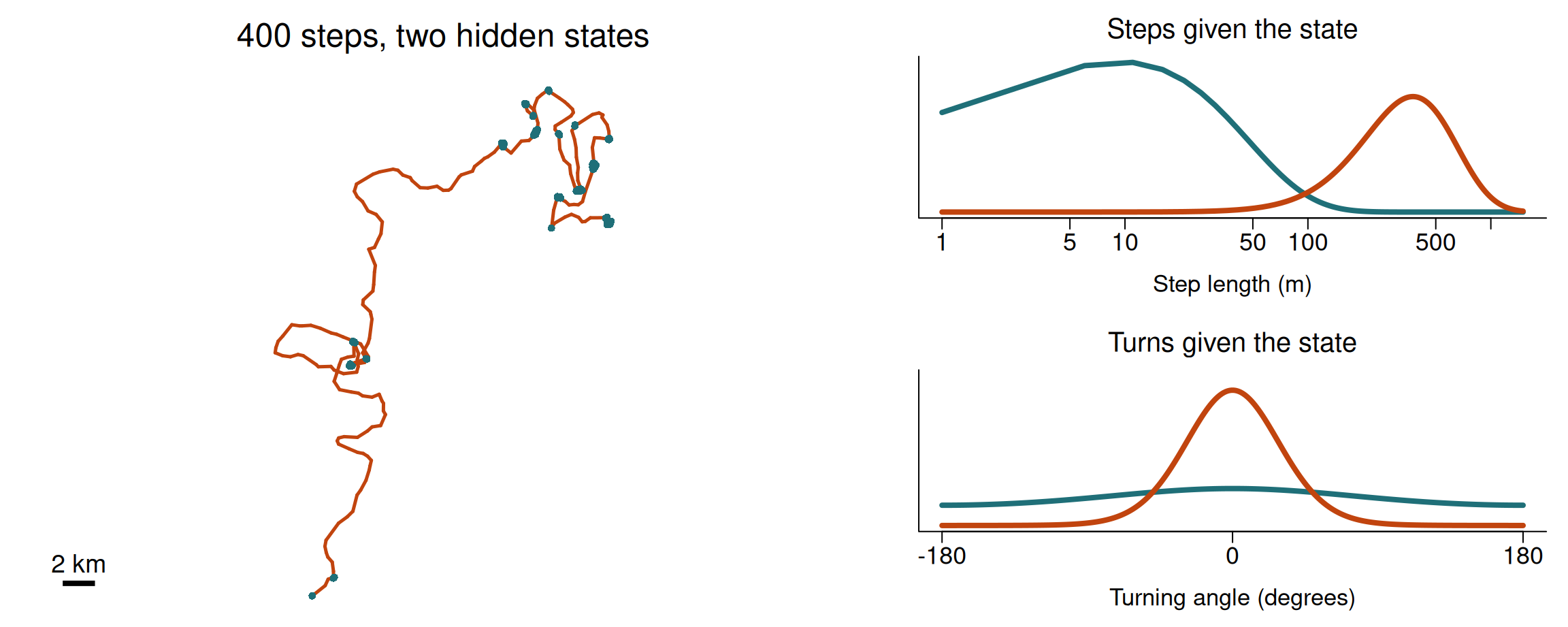
Teal: an encamped state, short steps and random turns. Red: a travelling state, long and directed. The HMM sees only the path and has to work out the colours.

What you get out

State-dependent parameters — e.g. state 1: mean step 40 m, turning angles ~uniform; state 2: mean step 600 m, angles concentrated at 0
Transition probability matrix \(\Gamma\) — and from it the expected dwell time in each state, \(1/(1-\gamma_{ii})\)
The most likely state sequence (Viterbi) — one label per step
State probabilities per step — the honest version, with uncertainty

m <- momentuHMM::fitHMM(data, nbStates = 2,
        dist = list(step = "gamma", angle = "vm"),
        Par0 = list(step  = c(20, 400, 20, 400),   # means, then sds
                    angle = c(0.5, 2)))            # concentrations
viterbi(m)

Two states in real buffalo

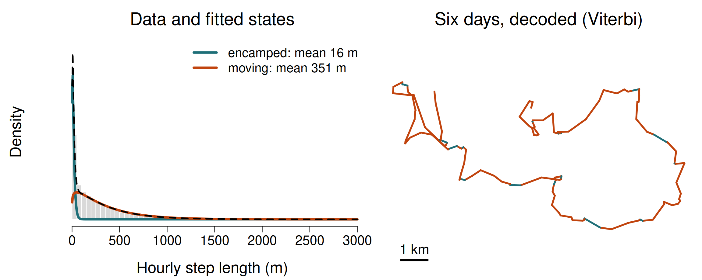
Cilla and Toni, hourly. Grey: all their steps. Coloured: the two fitted state distributions, weighted by how often each state occurs; dashed: their sum.

Why the Markov part matters

A clustering method looks at each step in isolation. An HMM knows that behaviour persists: an animal that was resting is probably still resting.

This borrows strength across time and produces far less “flickering” between states
The transition matrix is itself biology: how long does a foraging bout last?
Transitions can depend on covariates: is the animal more likely to start travelling when NDVI is low?

fitHMM(data, nbStates = 2, ..., formula = ~ ndvi + cosinor(hour, period = 24))

That formula is the bridge between Session 3’s environmental annotation and this one.

Flicker versus persistence

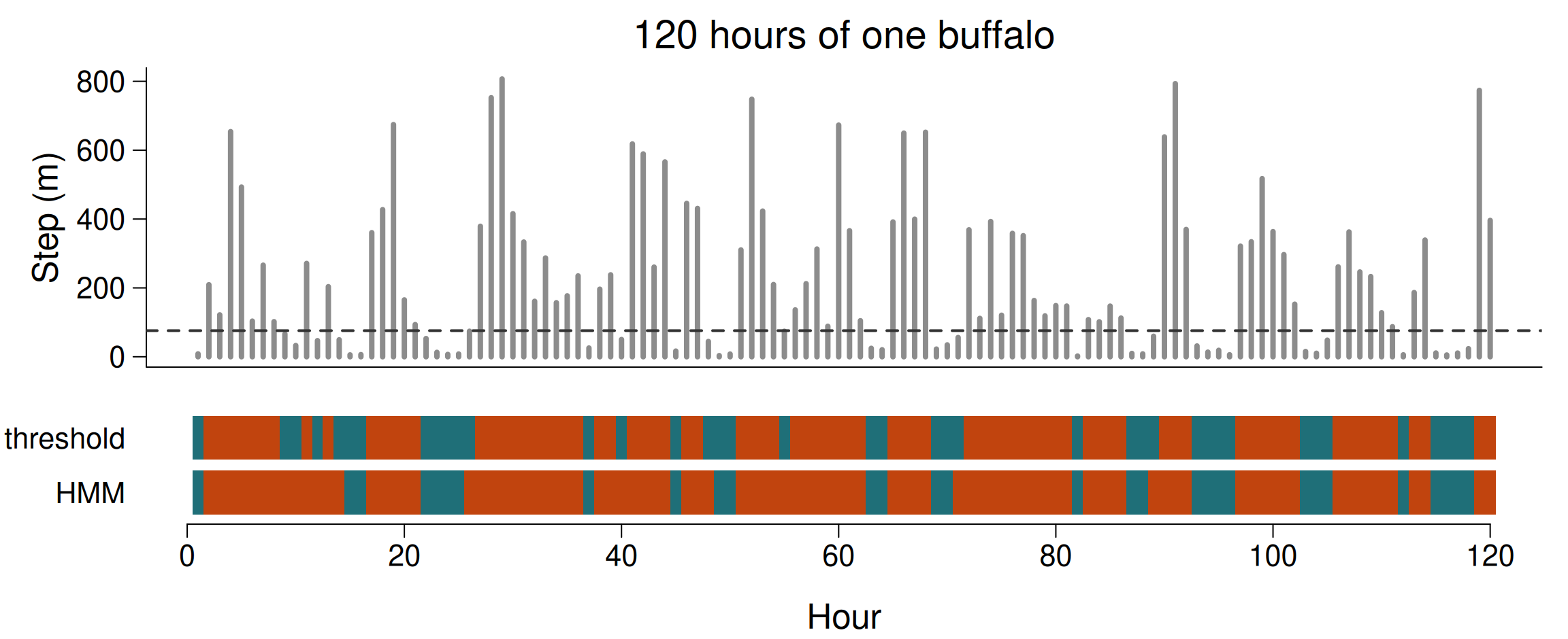
The same steps labelled two ways: a fixed threshold (dashed line) switches 35 times; the HMM, which knows that behaviour persists, 27 times.

Quiz

An HMM fitted to hourly buffalo data returns two states: state 1 with mean step 45 m, state 2 with mean step 780 m. The diagonal of the transition matrix is 0.93 and 0.86. What is the expected dwell time in state 2?

0.86 hours
About 7 hours
14 hours
Cannot be determined from the transition matrix alone

For a Markov chain the expected number of consecutive steps in state \(i\) is \(1/(1-\gamma_{ii})\). Here \(1/(1-0.86) \approx 7.1\) steps, and since steps are hourly, about 7 hours.

State 1 gives \(1/(1-0.93) \approx 14\) steps, i.e. ~14 hours — plausibly the resting/ruminating state.

Note two things. First, the dwell time depends on the sampling interval: the same animal sampled every 2 hours would give a different \(\gamma_{ii}\) but a similar dwell time in hours. Second, this is a real, checkable prediction — if the model says foraging bouts last 7 hours and you know from direct observation they last 45 minutes, the model is telling you your states are not what you think.

2 · Why not just a threshold?

Three things a threshold cannot do

Quantify uncertainty — an HMM gives every step a probability of being in each state, not a hard label. Steps near the boundary are honestly ambiguous
Use persistence — behaviour lasts; the transition matrix lets neighbouring steps inform each other, so a single slow step in the middle of a journey is not labelled “resting”
Explain switching — covariates on the transition probabilities ask when and where animals change behaviour

In Session 4 the buffalo’s hourly speeds had no valley to cut at. That is exactly the situation an HMM was built for.

A diel rhythm, estimated

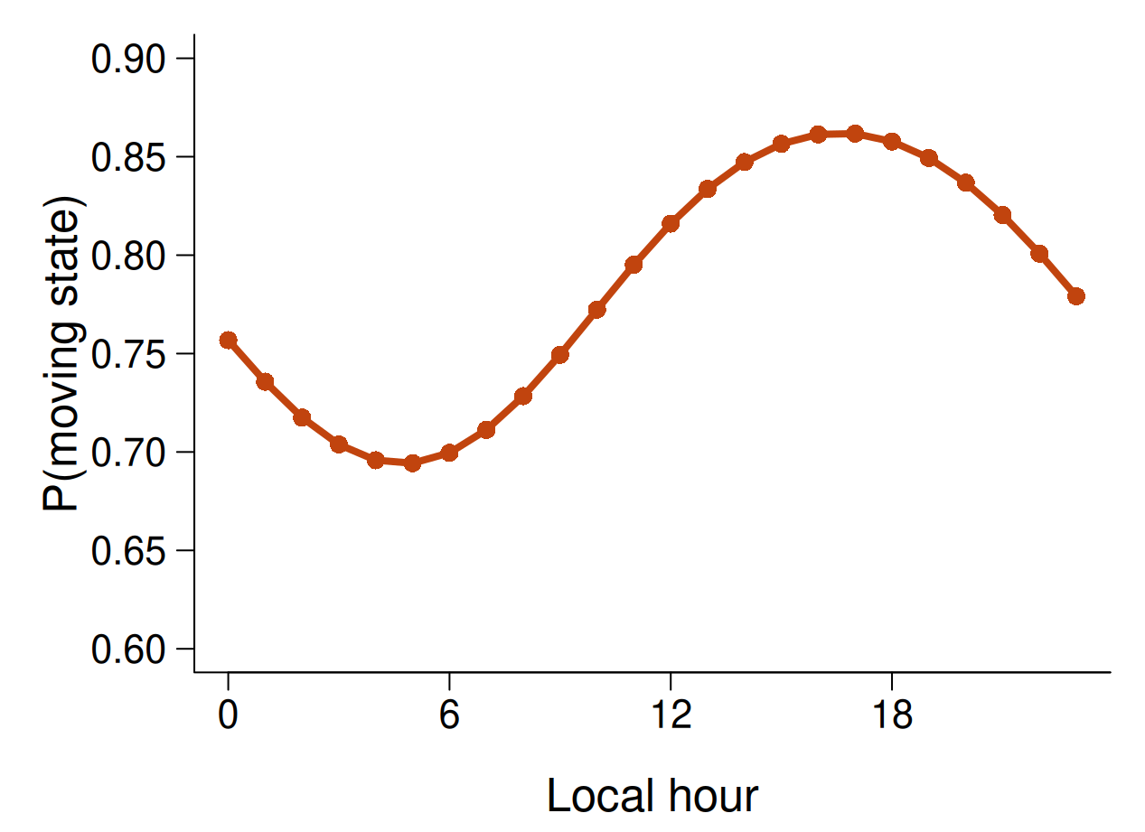
For two Kruger buffalo, a 2-state HMM with a daily cosinor on the transitions (hourly fixes, local time):

Local time	P(moving)
05:00	~0.69
11:00	~0.80
15:00–18:00	~0.86
23:00	~0.78

The covariate is on the switching, not on the step lengths: the buffalo do not walk differently in the afternoon, they are more likely to be walking. You fit this model in today’s practical.

3 · Where it goes wrong

Problem 1 — irregular sampling

HMMs as normally fitted assume a constant time step.

Feed them irregular data and the step-length distribution mixes intervals; the model interprets a long gap as fast movement
“Solutions” that are not solutions: interpolating to a regular grid invents data and biases the state distributions
Real solutions: resample and accept the data loss (Session 3); or use a continuous-time model (ctmm, momentuHMM with crawlWrap)

This is why the bat dataset cannot be given an HMM: 165 bursts with a median of 4 fixes cannot inform a transition matrix (Session 3).

Problem 2 — how many states?

AIC and BIC almost always prefer more states. They are answering “which model fits best”, not “which states are real behaviours”
With enough data, 4 and 5 states will beat 2 and 3 every time
Extra states often capture outliers, or the shape of the step-length distribution, not behaviour

Choose the number of states from biology and the question, then check the fit. Pseudo-residuals and state-dependent distribution plots tell you far more than a table of AICs. Two or three states are almost always enough for what a tracking dataset can actually resolve.

Quiz

You fit 2-, 3-, 4- and 5-state HMMs. AIC decreases every time. Which do you report?

The 5-state model — lowest AIC
The simplest model whose states are biologically interpretable and whose residuals are acceptable
Always 2 states, for comparability
Average the predictions across all four

AIC will keep improving because extra states always fit the shape of the data better — they mop up outliers and the tails of the step-length distribution. That is a statement about the flexibility of mixture models, not about the animal’s ethogram.

The defensible procedure: decide how many behavioural modes your data could plausibly resolve given the sampling interval, fit that model, and then check it — pseudo-residuals, state-dependent densities against the data, and dwell times against what you know about the species.

If a 4-state model gives you two states with nearly identical parameters, that is the model telling you it has run out of behaviour to find. Report the simpler one, and say why.

Problem 3 — naming the states

The model returns state 1 and state 2. It does not return “foraging” and “travelling”.

Labelling them is an interpretation, and it needs external evidence: accelerometer data, direct observation, known behaviours at known times
“Short steps and random turns” is consistent with foraging — and with resting, with sheltering, and with the animal being dead
Papers that name states from step lengths alone are making an assumption, not a measurement

State the evidence for your labels, or call them “state 1” and “state 2” and describe them by their parameters.

Quiz

Your 2-state HMM gives state 1 a mean step of 15 m with near-uniform turning angles. You want to call it “foraging”. What is the minimum you need?

Nothing — short steps with random turns is the standard definition of foraging
External evidence, because resting, sheltering and a dead animal all produce the same signature
A lower AIC than the 3-state model
A larger sample of animals

The model returns state 1, not foraging. Short steps with unstructured turning angles are consistent with foraging — and equally with resting, ruminating, sheltering from heat, a collar that fell off, and an animal that has died. At 15 m, a good part of the apparent movement is GPS error.

To turn the label into a measurement you need something outside the trajectory: accelerometer or activity data, direct observation, known diel patterns, or a validation subset with ground-truthed behaviour.

Where you have none, the honest write-up describes states by their parameters — “a low-displacement state (mean step 15 m, dwell time ~14 h)” — and discusses the plausible behaviours without asserting one.

Practical fitting advice

Starting values matter a lot. The likelihood is multimodal. Fit from many random starts and keep the best
Check for zero step lengths — a gamma distribution cannot handle them. Give momentuHMM one zero-mass parameter per state: a zero-inflated gamma
Always inspect pseudo-residuals (plotPR) — they are the residual plot of the HMM world
Plot the state-dependent densities over the histogram of your data. If they do not look like your data, nothing downstream is trustworthy

What checking looks like

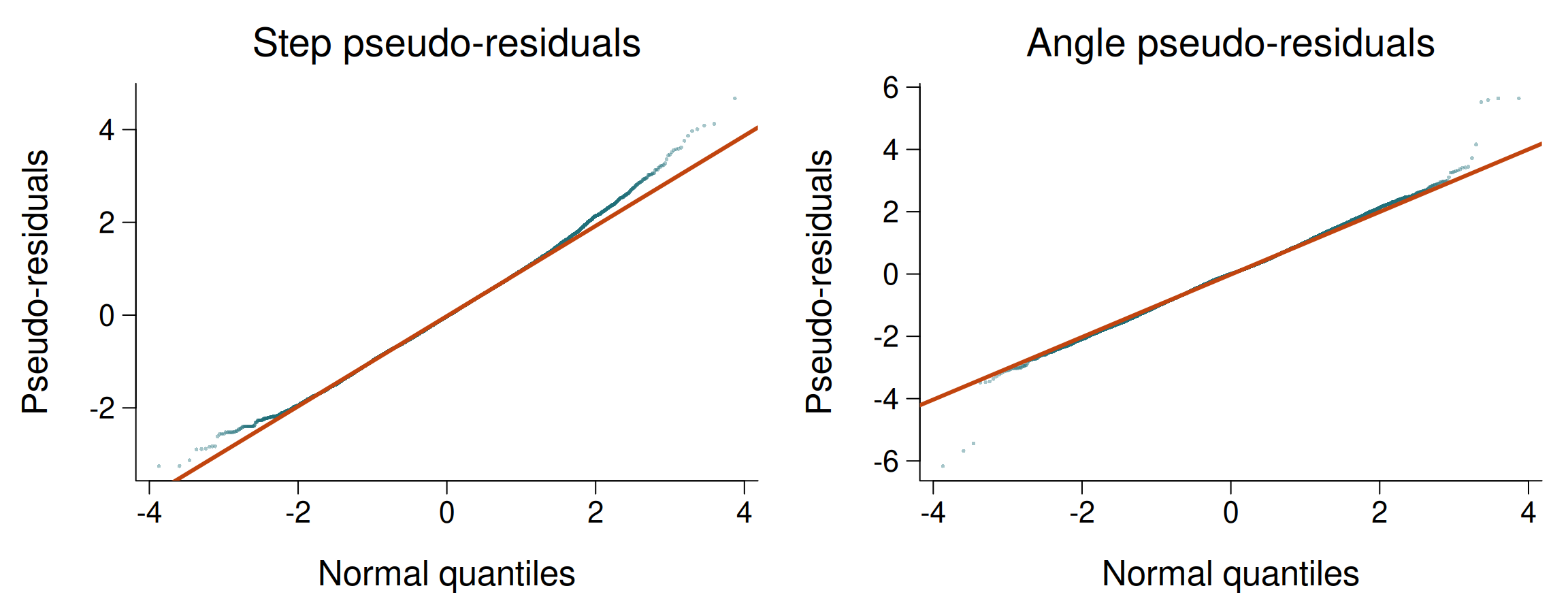
The two-state buffalo model. Points on the line mean the model describes the data; the bent tails of the step residuals say two states do not capture the full range of step lengths.

4 · The frontier

Location error, modelled

An HMM assumes the positions are exact. State-space models add an explicit observation layer: a true, unobserved path, and noisy fixes of it (Jonsen et al. 2005)
Essential for Argos and light-level geolocation, where error is as large as the movement
Continuous-time versions (crawl: Johnson et al. 2008) handle irregular sampling and predict positions with uncertainty — the honest version of interpolation from Session 3

Energy landscapes

The cost of moving is not the same everywhere: slope, wind, currents, thermals, substrate
An energy landscape maps that cost (Wilson et al. 2012; Shepard et al.
Animals often choose the cheap path, not the short one: soaring birds follow thermals and ridges; ungulates avoid steep ground
With accelerometers you can estimate energy expenditure directly and ask whether routes minimise it

Motion capacity becomes a map — and a covariate you can put in an SSF.

Collective movement

Animals rarely move independently: herds, flocks, schools, family groups
Simple local rules — attraction, alignment, repulsion — produce coordinated groups; a few informed individuals can steer many (Couzin et al. 2005)
Tracking several group members at once reveals who leads, who follows, and how decisions are made
Statistically: your “independent” animals may not be. Six buffalo from one herd are not six replicates

Learning behaviour from sensors

Tri-axial accelerometers at 10–50 Hz record what the body is doing
Supervised machine learning — random forests, support vector machines, and now deep neural networks — classify behaviours from acceleration signatures (Nathan et al. 2012; Wang 2019)
Training data come from observed or captive animals with known behaviour
The answer to “how do I name my HMM states?” — an independent sensor that measures behaviour

A classifier is only as good as its labelled training data, and it transfers poorly between individuals, seasons and populations. Validate on animals it has not seen.

The big-data era

Movebank holds billions of locations from thousands of studies; the ICARUS initiative put tracking receivers in orbit
Collaborative networks (e.g. EUROMAMMALS) pool data across studies, countries and decades
Questions no single study could answer: how movement responds to human footprint across continents; how migration changes with climate (Nathan et al. 2022)
New problems: data standards, sharing, credit, and the security of sensitive species

The skills of this course — cleaning, regularising, honest uncertainty — are what make pooled data trustworthy. At scale, errors compound too.

Quiz

You classify foraging behaviour of a seabird from accelerometer data with a random forest trained on birds filmed at one colony, and it scores 94% accuracy on held-out segments from those same birds. What should you worry about before applying it to a different colony?

Nothing — 94% is excellent
Accuracy measured on the training individuals overstates how well it transfers to new birds and places
Random forests cannot classify behaviour
The sampling frequency is too high

Held-out segments from the same birds share each bird’s idiosyncrasies — tag placement, body size, local conditions — so the test is not independent. Performance typically drops, sometimes sharply, on new individuals, seasons or colonies. Validate with whole individuals (and ideally whole sites) left out, exactly as for the habitat-selection models of Session 7.

The course, in one slide

What you have learned to do

Choose a technology and a fix interval, and name their biases (1)
Handle spatial data without lying about coordinate systems (2)
Clean a track, count what you removed, annotate it in space and time (3)
Quantify a path, and doubt your classifications (4)
Simulate a null, and a ground truth (5)
Estimate space use, and say which question the estimate answers (6)
Model selection and movement together (7)
Infer behavioural states, and supply the evidence for their names (8)

Six habits worth keeping

Look at the data before modelling it. Plot coordinates against time. Plot step length against time gap. Every dataset in this course had a defect you could see in one plot.
Count what you remove, at every step, and put the table in the paper.
Check that an argument did what you think. buffer= was silently ignored; group_by() was silently ignored. Both cost us most of a dataset.
Test your method on a truth you know. Simulate it first.
State your availability domain. Half of habitat-selection disagreements are definitional.
Report effect sizes, not p-values. You chose the sample size.

Your mini-project

One dataset, one clear question
Today: a 3–5 minute pitch — question, data, method, the pitfall you expect
Then a reproducible Quarto report: question → cleaning → analysis → figures → limitations. Submit the .qmd and the rendered HTML
See the syllabus for the marking criteria

The paragraph on limitations is worth more marks than the analysis. Anyone can run fit_issf(). Knowing what it cannot tell you is the skill.

Mini-project pitches

3–5 minutes each, no more than three slides

The question — one sentence, answerable with the data
The data — which dataset, which animals, what sampling interval
The method — which session’s tools, and why they fit the question
The pitfall — what could make your answer wrong, and how you will check

Examples: “compare home-range estimates under two fix rates using simulated data”; “SSF for a second fisher — does forest selection hold?”; “do the buffalo’s HMM states match day and night?”

Thank you

giuliano.colosimo@uniroma2.it

All material: github.com/GiulianoColosimo/animtrack-2627

Go and track something.