Simple feature collection with 2 features and 3 fields
Geometry type: POINT
Dimension:     XY
Bounding box:  xmin: 31.76 ymin: -24.54 xmax: 31.8 ymax: -24.5
Geodetic CRS:  WGS 84
  id   lon    lat             geometry
1  a 31.76 -24.54 POINT (31.76 -24.54)
2 b 31.80 -24.50 POINT (31.8 -24.5)Spatial data in R: the survival kit
Session 2 — Introduction to spatial data in R (sf, terra, projections)
Giuliano Colosimo
University of Rome Tor Vergata
2026-10-06
Today
Internal state Motion capacity Navigation capacity External factors Movement path
Today is about the two boxes we can actually measure: where the animal was (the path) and what was there (the environment). Everything later joins them.
Where we are going
- Vector vs raster, and when each is appropriate
- Coordinate reference systems — and why distances in lat/long are wrong
- Choosing a projection for the analysis you are about to do
- Why the R spatial stack changed, and what that means for old code
sffor vectors,terrafor rasters, and the verbs that join them- Where environmental rasters come from: a remote-sensing primer
This is the standalone “intro to spatial R” session. It is worth having even if you never analyse another track.
1 · Two ways to represent the world
Vector and raster
Vector
Discrete objects with coordinates.
- Point — a fix, a nest, a trap
- Line — a trajectory, a river, a road
- Polygon — a home range, a park boundary, a lake
Each object carries an attribute table.
Exact geometry, arbitrary precision.
Raster
A regular grid of cells, each with a value.
- Elevation, NDVI, temperature, land cover
- Defined by origin, cell size, number of rows/cols, CRS
Continuous surfaces, fixed resolution.
Fast maths, no notion of individual objects.
Movement analysis is nearly always points (or steps) sampling rasters. That one sentence describes Sessions 3 and 7.
The same place, both ways
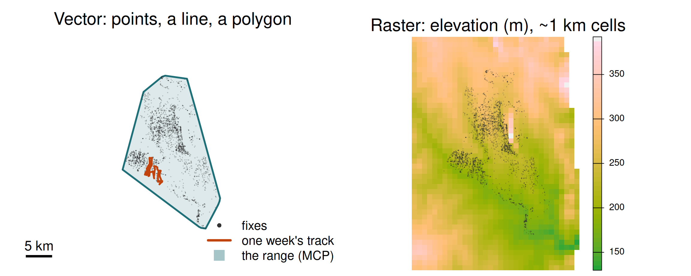
Cilla’s fixes, one week of her track and her range as vectors; the terrain under them as a raster.
Choosing the model
| Question | Model |
|---|---|
| Where exactly was the animal at 08:00? | Vector (point) |
| What is the NDVI there? | Raster, sampled at that point |
| What is the park boundary? | Vector (polygon) |
| How far is the nearest river? | Raster (a distance surface) or vector + distance computation |
| How much forest within 500 m? | Raster, summarised in a buffer |
The same reality can be either. A river is a line if you care about its course, and a distance-to-river raster if you care about how far the animal is from it. Choose by the operation you need, not by what the thing “is”.
2 · Coordinate reference systems
The problem
The Earth is a lumpy ellipsoid. Maps and computer screens are flat. Getting from one to the other requires choices, and every choice distorts something.
A CRS answers three questions:
- What shape is the Earth? — the ellipsoid (e.g. WGS84, GRS80)
- How is that shape tied to the actual planet? — the datum
- How do we flatten it? — the projection (or none, if we keep angles)
Geographic coordinates
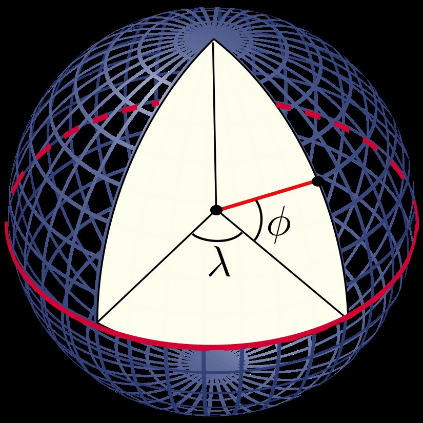
Longitude and latitude are angles, not distances
Latitude: angle north/south of the equator. Longitude: angle east/west of Greenwich. Units are degrees. This is what every GPS and every Movebank file gives you — usually WGS84, EPSG:4326.
Why you cannot do arithmetic with degrees
- One degree of latitude ≈ 111 km everywhere
- One degree of longitude ≈ 111 km × cos(latitude)
- at the equator: 111 km
- at 24° (Kruger): ~102 km
- at 46° (Switzerland): ~77 km
- at the pole: 0 km
Euclidean distance on longitude/latitude is meaningless. You either project to a metric CRS, or compute great-circle distances on the ellipsoid. sf does the second automatically for EPSG:4326 — which is safe, but slower, and does not fix your plots.
One degree is not one distance
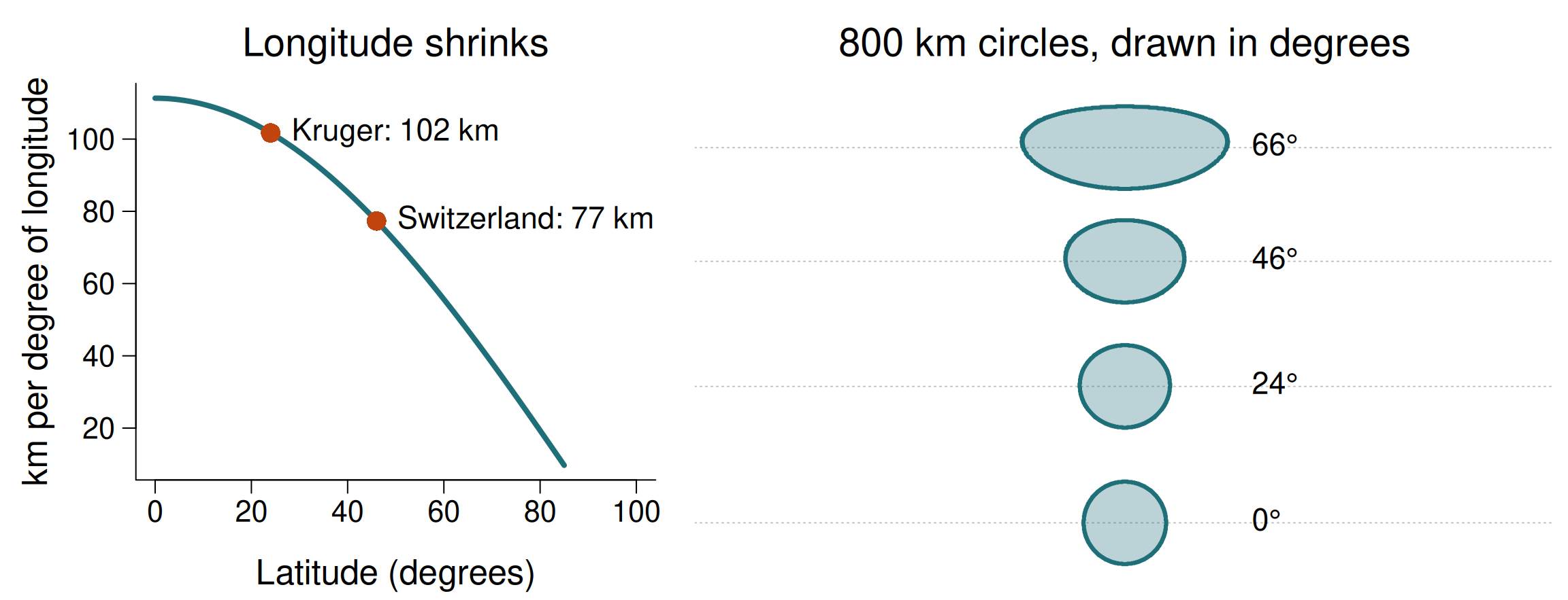
Every circle has an 800 km radius on the ground. Plotted as if degrees were metres, they stretch east–west — badly at high latitudes.
Projected coordinates
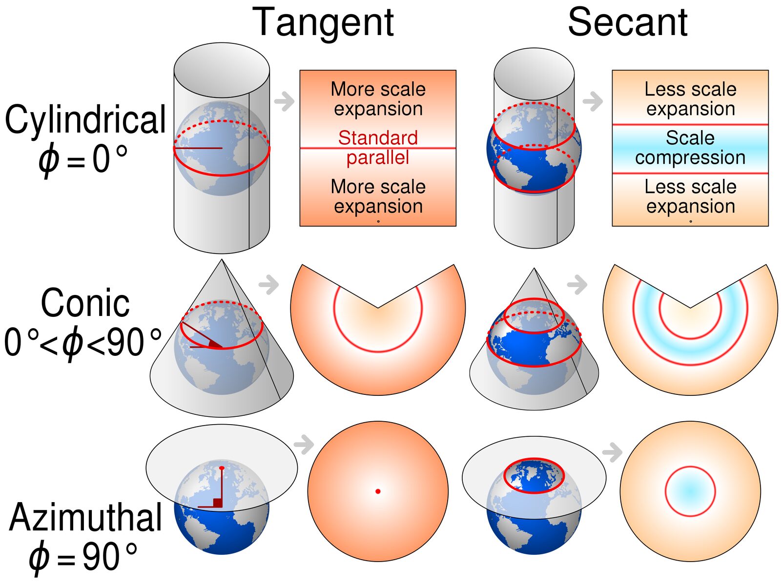
Every projection preserves some properties and destroys others
Conformal keeps angles/shape (Mercator, UTM). Equal-area keeps area (Albers, Mollweide). Equidistant keeps distances from a point. No projection keeps everything.
UTM: the practical default
- The world is cut into 60 zones, each 6° of longitude wide
- Each zone gets its own transverse Mercator projection, so distortion inside a zone is small (< 0.1%)
- Coordinates in metres: easting and northing
- Kruger is in zone 36S → EPSG:32736
- Switzerland is in zone 32N → EPSG:32632
UTM works beautifully inside one zone. Leo the vulture crosses many zones and 47° of latitude, so no single UTM zone fits him. For continental-scale tracks use an equal-area CRS suited to the region — or work in geographic coordinates with geodesic distances.
Choose the projection for the analysis
No projection preserves everything, so pick the property your analysis needs:
| You will compute… | Preserve… | Typical choice |
|---|---|---|
| Step lengths, distances | distance | local UTM zone, or azimuthal equidistant centred on the study area |
| Home-range areas, densities | area | Albers or Lambert equal-area (LAEA) |
| Directions, turning angles | angles / shape | conformal: UTM (locally) |
| A continent-scale migration | area, usually | LAEA centred on the flyway |
Inside one UTM zone the distortions are under 0.1%, so UTM does all three well enough. The choice only becomes real when your animal leaves the zone.
EPSG codes — the vocabulary you need
| EPSG | What | Units |
|---|---|---|
| 4326 | WGS84 geographic — GPS, Movebank | degrees |
| 3857 | Web Mercator — Google/OSM basemaps. Never for analysis | metres |
| 32736 | UTM zone 36S — Kruger | metres |
| 32632 | UTM zone 32N — Switzerland, Italy | metres |
| 3035 | ETRS89 / LAEA Europe — equal-area, continental | metres |
| 6933 | WGS84 / NSIDC EASE-Grid 2.0 Global — equal-area, global | metres |
3857 is a trap. It is conformal, wildly non-equal-area, and areas near the poles are inflated by orders of magnitude. Use it to display tiles, never to compute a home range.
The same circles, two projections
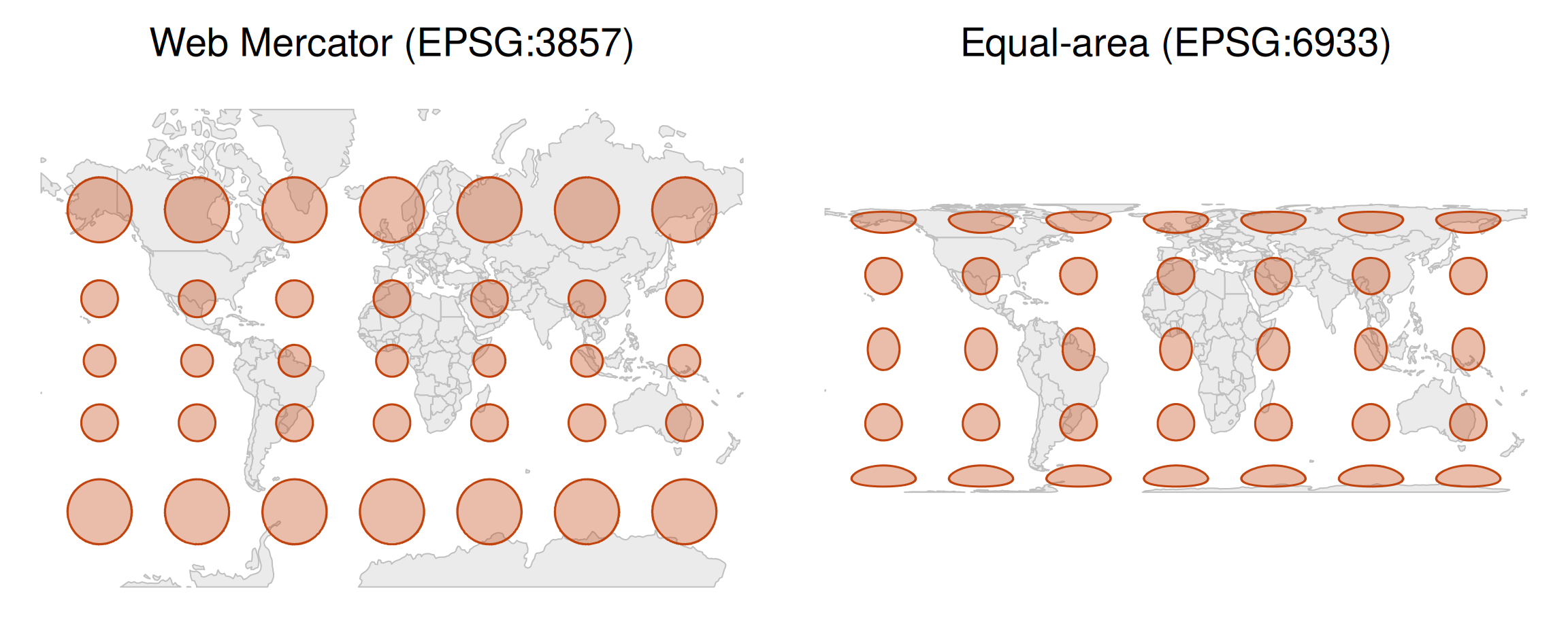
Every red disc covers the same 2.5 million km². Web Mercator inflates them towards the poles; an equal-area projection keeps their areas equal, at the cost of their shapes.
Quiz
You have buffalo fixes in EPSG:4326 and you want the area of a 95% home range polygon, in km². What is the right sequence?
Project first, to a CRS whose units are metres and which is appropriate for the region — UTM 36S for Kruger. Then all the geometry operations are ordinary plane geometry and areas come out in m².
There is no fixed conversion from degrees² to km²: the factor depends on latitude. Web Mercator (3857) has units of metres but is not equal-area, so areas are systematically wrong. And while sf can compute geodesic lengths and areas on 4326, kernel-density home-range estimators need projected coordinates — they assume a plane.
3 · A short, messy history
Why your old tutorial no longer runs
| Era | Vector | Raster | Geometry engine |
|---|---|---|---|
| 2005–2023 | sp |
raster |
rgdal, rgeos |
| 2016 → | sf |
sf (GDAL, GEOS, PROJ built in) |
|
| 2020 → | terra |
terra |
rgdal,rgeosandmaptoolswere retired from CRAN in October 2023;rasternow runs on top ofterra- Most Stack Overflow answers and many published scripts still use
sp/raster - Some movement packages —
adehabitatLT,adehabitatHR— still expectspobjects. You will convert withas(x, "Spatial")orsf::as_Spatial()
Write new code in sf + terra. Recognise sp + raster when you read it.
4 · sf — vector data
The idea behind sf
A simple feature data frame is an ordinary data frame with one extra column, geometry, that holds the coordinates — and a CRS attached.
Everything else is dplyr
Because it is a data frame, all your usual verbs work, and the geometry comes along for the ride.
Simple feature collection with 1 feature and 2 fields
Geometry type: POINT
Dimension:     XY
Bounding box:  xmin: 31.8 ymin: -24.5 xmax: 31.8 ymax: -24.5
Geodetic CRS:  WGS 84
  id label           geometry
1  b     B POINT (31.8 -24.5)
Note the geometry column survives select() without being named — it is “sticky”. Use st_drop_geometry() when you genuinely want a plain data frame.
The functions you will actually use
| Function | What it does |
|---|---|
st_as_sf() |
data frame → spatial |
st_crs() |
get/set the CRS. Setting ≠ transforming |
st_transform() |
reproject to another CRS |
st_coordinates() |
pull the coordinates back out as a matrix |
st_distance() |
distances between features |
st_buffer() |
a polygon at a fixed distance around features |
st_join() |
attach attributes of the polygon each point falls in |
st_bbox() |
bounding box |
st_intersection(), st_union() |
overlay operations |
st_write() / st_read() |
GeoPackage, shapefile, GeoJSON… |
st_crs() vs st_transform() — the classic bug
st_crs(x) <- 32736
“These numbers were always UTM; I am just writing down the label.”
If the numbers are actually degrees, you have now lied to R. Your buffalo are now in Antarctica (next slide).
st_transform(x, 32736)
“These numbers are in the current CRS; compute the corresponding UTM coordinates.”
The numbers change. This is almost always what you want.
Assign a CRS only when the data arrived without one and you know what it should be. Otherwise, transform.
Where the mislabelled buffalo went
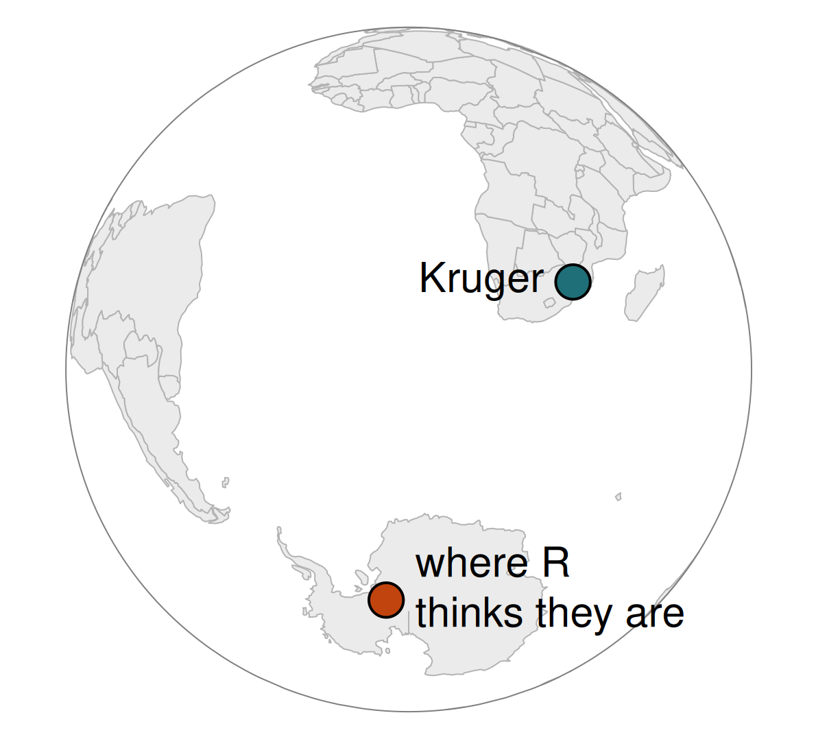
(31.76, −24.54) read as metres in UTM 36S is a spot 31 m east and 24 m south of the zone’s false origin: 500 km west of the 33°E meridian and 10,000 km south of the equator.
That is (57°W, 85.5°S) — the Antarctic ice sheet. No error, no warning.
Quiz
Your colleague sends a CSV of coordinates like x = 375051, y = 7285726 and says “they’re from Kruger”. What are they, and what do you do?
Magnitudes give it away. Longitude and latitude are bounded by ±180 and ±90, so six- and seven-digit values cannot be degrees. Values of that size in metres with a large northing are classic UTM, and Kruger is zone 36S (EPSG:32736) — the 7,285,726 m northing is the southern-hemisphere false northing at ~24.5°S.
Because the numbers are already UTM, you declare the CRS when building the sf object (crs = 32736) rather than transforming. Transforming would treat metres as degrees.
Sanity check afterwards: st_transform(x, 4326) and confirm you land at roughly 31.8°E, 24.5°S.
5 · terra — raster data
A raster is a grid plus metadata
class       : SpatRaster
size        : 4, 6, 1  (nrow, ncol, nlyr)
resolution  : 0.1, 0.1  (x, y)
extent      : 31.5, 32.1, -24.8, -24.4  (xmin, xmax, ymin, ymax)
coord. ref. : lon/lat WGS 84 (EPSG:4326)
source(s)   : memory
name        : lyr.1
min value   :     1
max value   :    24
What defines a raster
- Extent — xmin, xmax, ymin, ymax
- Resolution — cell size in CRS units.
res(r) - Dimensions — rows × columns × layers.
dim(r) - CRS — same concept as for vectors
- Values — one per cell per layer, possibly
NA
A multi-layer raster (SpatRaster with several layers) is how you store a time series: one NDVI layer per 16-day composite, stacked. That is exactly what we need in Session 3.
The terra functions you will use
| Function | What it does |
|---|---|
rast() |
create or read a raster |
crop() / mask() |
cut to an extent / to a polygon |
project() |
reproject (note: not st_transform) |
extract() |
sample raster values at points — the key operation |
aggregate() / resample() |
change resolution |
terrain() |
slope, aspect, from elevation |
distance() |
distance-to-feature surface |
global(), zonal() |
summaries |
writeRaster() |
save, usually GeoTIFF |
extract() is the bridge between the movement world and the environment world. Almost everything from Session 3 onwards passes through it.
Rasters and vectors must agree
Before extract(), three things must line up:
- Same CRS. If both objects carry a CRS,
terratransforms for you and warns. If either lacks one — a bare coordinate matrix — it assumes they match. - Overlapping extents. Non-overlap gives you a column of
NA, not an error. - Appropriate resolution. Extracting a 1 km NDVI cell for a fix with 10 m GPS error is fine. Extracting a 10 m Sentinel pixel for an Argos fix with 5 km error is self-deception.
Match the resolution of your environmental data to the error of your locations. A pixel finer than your positional error adds noise, not information.
Quiz
You run terra::extract(ndvi, cbind(buffalo$lon, buffalo$lat)) and every value comes back NA. The NDVI raster is in UTM 36S. What happened?
Modern terra is helpful when it can be: give it a SpatVector or an sf object that carries a CRS, and it transforms your points for you, printing a warning:
[extract] transforming vector data to the CRS of the rasterBut a plain two-column matrix has no CRS. terra can only assume the numbers are already in the raster’s coordinate system — so 31.8 and −24.5 are read as metres, land far outside the extent, and every lookup returns NA.
The same silent failure happens if the CRS of either object is missing (crs(r) <- ""). Lesson: keep your data in objects that carry their CRS, and never strip coordinates down to a bare matrix just to pass them along.
6 · Where rasters come from
Why vegetation looks the way it does
Healthy green vegetation:
- absorbs strongly in the red (~660 nm) — chlorophyll is doing photosynthesis
- reflects strongly in the near infrared (~850 nm) — the internal leaf structure scatters it
So the contrast between red and NIR is a measure of green biomass.
That single fact is the basis of essentially every vegetation index ever published.
Spectral signatures
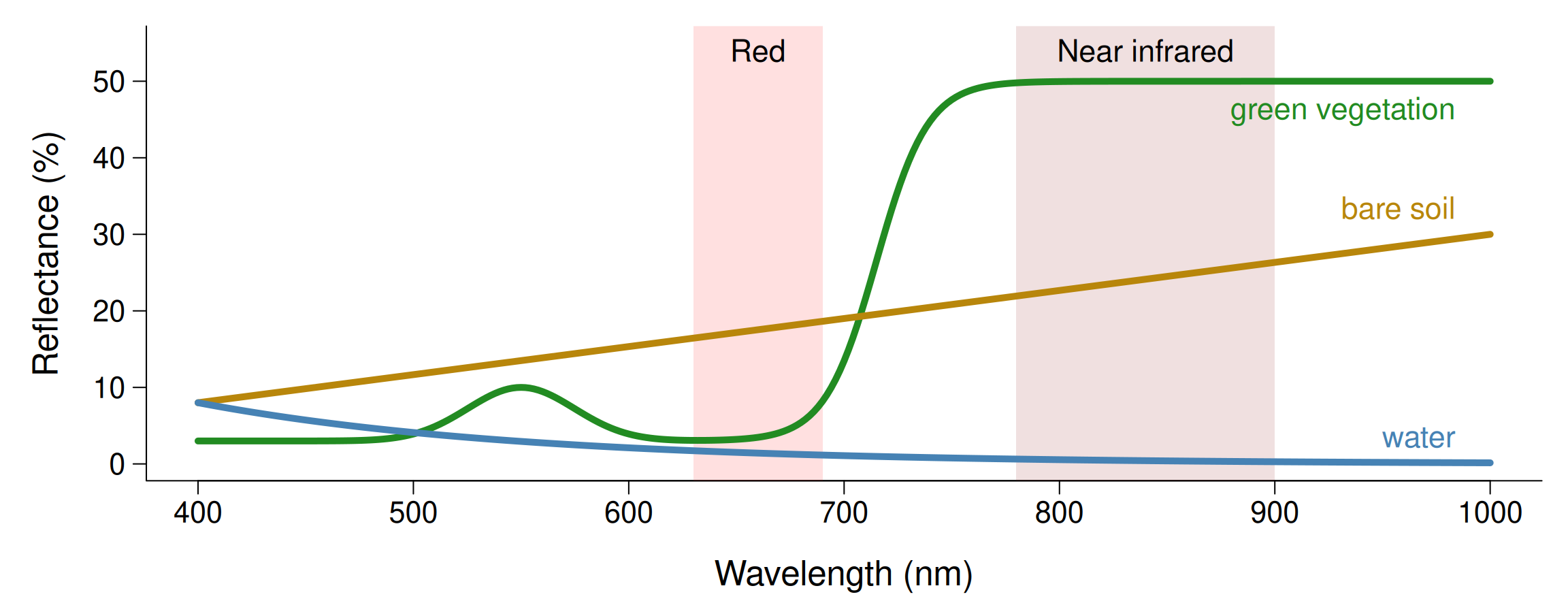
Schematic curves. Vegetation is dark in the red and bright in the near infrared; soil and water are not. NDVI measures exactly that contrast.
NDVI
\[\text{NDVI} = \frac{\text{NIR} - \text{Red}}{\text{NIR} + \text{Red}}\]
- Ranges −1 to +1. Water < 0; bare soil/rock ~0.1–0.2; sparse vegetation ~0.2–0.4; dense green vegetation 0.6–0.9
- A proxy for green biomass and primary productivity
- Normalised, so it partly cancels illumination and viewing-angle effects
It saturates. Above ~0.8 — closed canopy — NDVI stops responding to extra biomass. In rainforest it is nearly flat and nearly useless.
Kruger, wet and dry
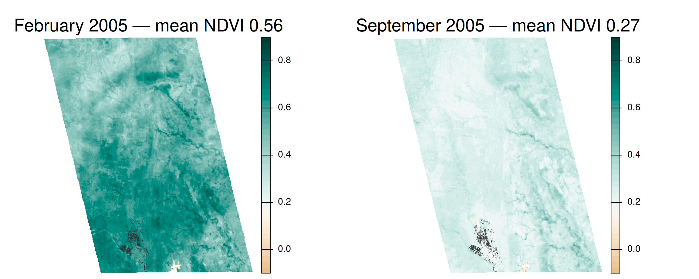
MODIS NDVI at 250 m, the same landscape six months apart (dots: Cilla’s fixes). An NDVI value is only meaningful together with its date.
You cannot have all four
- Spatial — pixel size. 10 m (Sentinel-2) … 500 m (MODIS) … 25 km (some climate products)
- Temporal — revisit time. 5 days (Sentinel-2) vs daily (MODIS) vs 16 days (Landsat)
- Spectral — number and width of bands. 4 broad bands vs 200 narrow (hyperspectral)
- Radiometric — bit depth; how finely brightness is quantised
They trade off against each other: a detector collecting light from a small patch, in a narrow band, gets few photons — so it needs a longer dwell time, which means a narrower swath and a longer revisit.
Pixel size changes the landscape
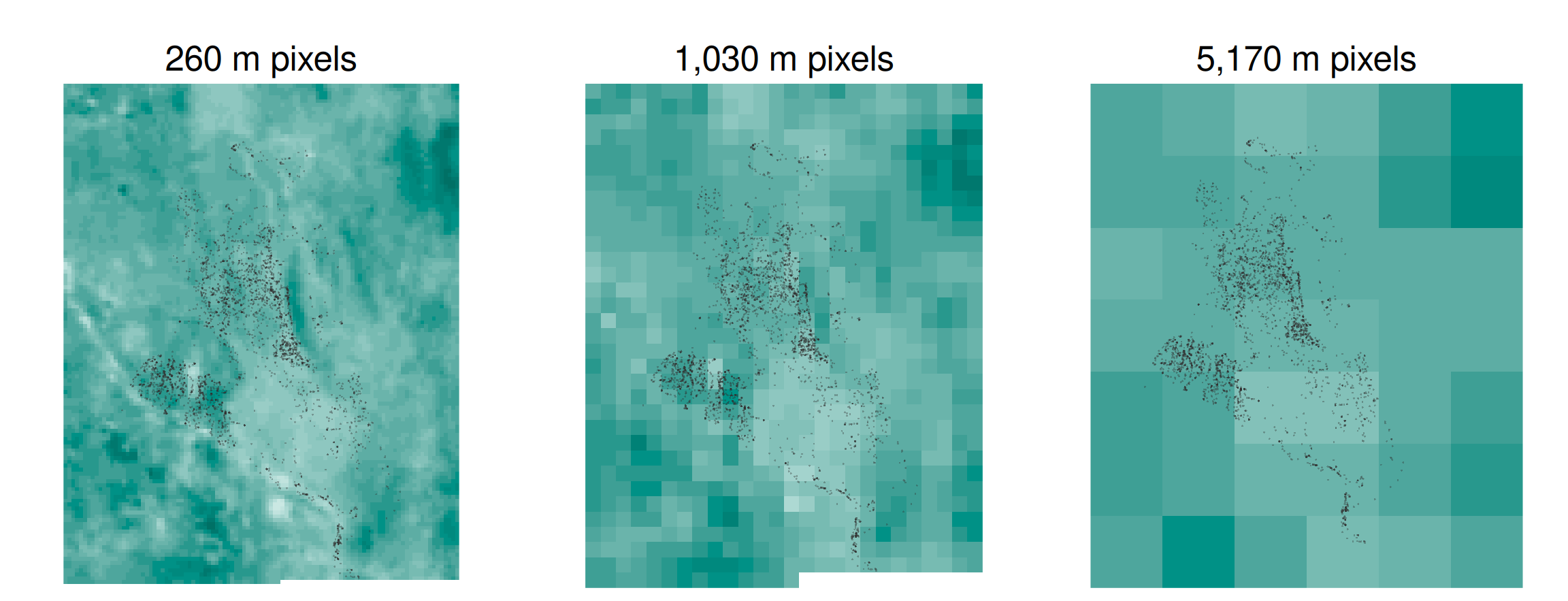
The same February NDVI around Cilla’s range at MODIS resolution, then averaged to ~1 km and ~5 km. At 5 km every fix gets nearly the same value.
The missions you will actually use
| Mission | Spatial | Temporal | Since | Good for |
|---|---|---|---|---|
| MODIS (Terra/Aqua) | 250–500 m | Daily | 2000 | Long consistent NDVI series |
| VIIRS | 375–750 m | Daily | 2012 | MODIS successor |
| Landsat 5/7/8/9 | 30 m | 16 days | 1984 | Long-term landscape change |
| Sentinel-2 | 10–20 m | 5 days | 2015 | Fine-grained habitat |
| Sentinel-1 (SAR) | 10 m | 6–12 days | 2014 | Cloud-free, structure, water |
| GEDI (LiDAR) | 25 m footprint | sampled | 2019 | Canopy height |
Match the pixel to the animal and to your positional error. A 10 m Sentinel pixel is wasted on an Argos fix with 5 km error — and a 500 m MODIS pixel is useless for a dormouse.
Quiz
You study habitat selection by a forest ungulate using GPS collars (error ~15 m, hourly fixes) in a landscape with small forest patches of 1–5 ha. Which product for vegetation cover?
A 1–5 ha patch is roughly 100–220 m across. A 250 m MODIS pixel is larger than the patch, so every fix would get a mixed value averaging forest and open land — the very contrast you are trying to measure would be erased. A 1 km product is hopeless for the same reason.
Sentinel-2 at 10–20 m resolves those patches comfortably, and its 5-day revisit captures the growing season. Its resolution is also well matched to 15 m GPS error: finer would just add noise.
Sentinel-1 is excellent for structure and for cloudy regions, but it does not measure greenness — it is the right answer to a different question.
Today’s practical
sf: build points from a CSV,st_transform,st_buffer,st_join,st_intersection- Measure one distance three ways — and get three answers
terra: load NDVI and land cover,crop,project,extract- Break it on purpose: the silent
NAand the ignored buffer - Mini-challenge: a publication-quality map with
geom_sf
Recap
- Vector = objects with coordinates; raster = a grid of values
- A CRS = ellipsoid + datum + projection. Degrees are angles
- Choose the projection for the analysis: equidistant for steps, equal-area for home ranges
sf+terratoday;sp+rasterin old codest_crs()labels;st_transform()converts- Satellites measure bands; NDVI is a red/NIR contrast. Match the pixel to your positional error
Before Session 3
- Read Geocomputation with R, ch. 2 and 7
- Make sure
library(amt)andlibrary(adehabitatLT)both load