Practical 2 — The spatial survival kit

Session 2 · Spatial data in R

Modified

September 30, 2026

Goals. Turn a CSV into an sf object; reproject it and measure distances correctly; use the vector verbs you will need all course (st_buffer, st_join, st_intersection); load real NDVI and land-cover rasters with terra and sample them at the fixes; break things on purpose; and finish with a publication-quality map.

Time: ~80 minutes. Packages: sf, terra, dplyr, ggplot2, ggspatial.

library(sf)
library(terra)
library(dplyr)
library(ggplot2)

Task 1 — From data frame to `sf`

track <- readr::read_csv("data/buffalo_kruger.csv.gz", show_col_types = FALSE) |>
  transmute(id = `individual-local-identifier`, t = timestamp,
            lon = `location-long`, lat = `location-lat`) |>
  filter(!is.na(lon), !is.na(lat)) |>
  distinct(id, t, .keep_all = TRUE) |>
  arrange(id, t)

fixes <- st_as_sf(track, coords = c("lon", "lat"), crs = 4326, remove = FALSE)
fixes
#> Simple feature collection with 24663 features and 4 fields
#> Geometry type: POINT
#> Dimension:     XY
#> Bounding box:  xmin: 31.58639 ymin: -25.16421 xmax: 32.35671 ymax: -23.99802
#> Geodetic CRS:  WGS 84
#> # A tibble: 24,663 × 5
#>    id    t                     lon   lat             geometry
#>  * <chr> <dttm>              <dbl> <dbl>          <POINT [°]>
#>  1 Cilla 2005-07-14 04:35:00  31.8 -25.1 (31.80449 -25.06147)
#>  2 Cilla 2005-07-14 05:35:00  31.9 -25.0 (31.88776 -24.96738)
#>  3 Cilla 2005-07-14 07:35:00  31.9 -24.9 (31.85942 -24.94288)
#>  4 Cilla 2005-07-14 08:34:00  31.9 -24.9 (31.85512 -24.94914)
#>  5 Cilla 2005-07-14 09:35:00  31.9 -25.0 (31.85694 -24.95424)
#>  6 Cilla 2005-07-14 10:35:00  31.9 -24.9 (31.85977 -24.94735)
#>  7 Cilla 2005-07-14 11:34:00  31.8 -24.9 (31.84466 -24.93435)
#>  8 Cilla 2005-07-14 12:35:00  31.8 -24.9    (31.8441 -24.934)
#>  9 Cilla 2005-07-14 13:34:00  31.8 -24.9 (31.84463 -24.93442)
#> 10 Cilla 2005-07-14 14:35:00  31.9 -24.9   (31.857 -24.93371)
#> # ℹ 24,653 more rows

Your turn

1a. What CRS is this, in what units? 1b. What is the bounding box?

Solution

st_crs(fixes)$epsg
#> [1] 4326
st_is_longlat(fixes)
#> [1] TRUE
st_bbox(fixes)
#>      xmin      ymin      xmax      ymax 
#>  31.58639 -25.16421  32.35671 -23.99802

EPSG:4326, degrees — and st_is_longlat() returning TRUE is the flag that should make you stop before computing any distance or area.

Task 2 — Reproject, and measure one distance three ways

Kruger is in UTM zone 36S, EPSG:32736.

fixes_utm <- st_transform(fixes, 32736)

queen <- fixes |> filter(id == "Queen") |> slice(1:2)
xy <- st_coordinates(queen)

wrong     <- sqrt(diff(xy[, 1])^2 + diff(xy[, 2])^2)          # "distance" in degrees
geodesic  <- st_distance(queen[1, ], queen[2, ])              # on the ellipsoid
projected <- st_distance(st_transform(queen, 32736)[1, ],
                         st_transform(queen, 32736)[2, ])     # in UTM metres

c(wrong_degrees = wrong, geodesic_m = as.numeric(geodesic),
  projected_m = as.numeric(projected))
#> wrong_degrees    geodesic_m   projected_m 
#>  2.835514e-03  3.014658e+02  3.009957e+02

What the three numbers mean

The first is not a distance at all: it mixes degrees of longitude and latitude, which are different lengths. The other two agree to a small fraction of a percent — UTM’s distortion inside a zone is under 0.1%.

For distances either works. For kernel densities, buffers and anything involving area, project first: those methods assume a plane.

Task 3 — Vector verbs: buffer, join, intersect

We need polygons to overlay. Build them from the land-cover raster: for each cell, which cover type dominates?

lc <- rast("data/kruger_landcover.tif")[[c("trees", "grassland", "shrubs")]]
dominant <- which.max(lc)
levels(dominant) <- data.frame(id = 1:3, cover = c("trees", "grassland", "shrubs"))

habitat <- as.polygons(dominant, dissolve = TRUE) |>
  st_as_sf() |>
  st_transform(32736)

habitat
#> Simple feature collection with 3 features and 1 field
#> Geometry type: MULTIPOLYGON
#> Dimension:     XY
#> Bounding box:  xmin: 337122.5 ymin: 7200872 xmax: 449667.9 ymax: 7356755
#> Projected CRS: WGS 84 / UTM zone 36S
#>       cover                       geometry
#> 1     trees MULTIPOLYGON (((387178.5 73...
#> 2 grassland MULTIPOLYGON (((411785.8 73...
#> 3    shrubs MULTIPOLYGON (((405848 7355...

`st_join()` — which polygon is each fix in?

fixes_hab <- st_join(fixes_utm, habitat)

fixes_hab |>
  st_drop_geometry() |>
  count(cover) |>
  mutate(share = round(n / sum(n), 3))
#> # A tibble: 3 × 3
#>   cover         n share
#>   <chr>     <int> <dbl>
#> 1 grassland 24090 0.977
#> 2 shrubs      476 0.019
#> 3 trees        97 0.004

`st_buffer()` and `st_intersection()` — what is around the animal?

cilla_area <- fixes_utm |>
  filter(id == "Cilla") |>
  st_buffer(dist = 500) |>          # 500 m around every fix
  st_union()                        # one polygon: the area Cilla came near

used_hab <- st_intersection(habitat, cilla_area) |>
  mutate(km2 = as.numeric(st_area(geometry)) / 1e6)

used_hab |> st_drop_geometry() |> select(cover, km2)
#>       cover        km2
#> 1     trees   2.424118
#> 2 grassland 221.503730
#> 3    shrubs   1.848077

Your turn

3a. Compare the habitat composition of Cilla’s area with that of the whole landscape. 3b. Why must habitat and cilla_area be projected here?

Solution

study <- st_as_sfc(st_bbox(habitat))
landscape <- st_intersection(habitat, study) |>
  mutate(km2 = as.numeric(st_area(geometry)) / 1e6)

left_join(
  landscape |> st_drop_geometry() |> transmute(cover, landscape = km2 / sum(km2)),
  used_hab  |> st_drop_geometry() |> transmute(cover, cilla = km2 / sum(km2)),
  by = "cover"
) |>
  mutate(across(c(landscape, cilla), \(z) round(z, 3)),
         ratio = round(cilla / landscape, 2))
#>       cover landscape cilla ratio
#> 1     trees     0.245 0.011  0.04
#> 2 grassland     0.424 0.981  2.31
#> 3    shrubs     0.331 0.008  0.02

A ratio above 1 means Cilla’s surroundings contain more of that cover than the landscape does. This used-versus-available comparison is the seed of Session 7.

Both layers must be projected because st_buffer(dist = 500) needs metres (in degrees, 500 would be absurd) and st_area() of a union of buffers assumes a plane. sf would compute geodesic areas on 4326, but buffering in degrees produces ellipses, not circles.

Task 4 — Rasters with `terra`: NDVI

data/kruger_ndvi_2005.tif holds two MODIS 16-day NDVI composites (MOD13Q1, 250 m) over the buffalo range: one from the wet season and one from the dry season of 2005.

ndvi <- rast("data/kruger_ndvi_2005.tif")
ndvi
#> class       : SpatRaster
#> size        : 481, 463, 2  (nrow, ncol, nlyr)
#> resolution  : 0.002432149, 0.002432149  (x, y)
#> extent      : 31.41276, 32.53885, -25.1657, -23.99583  (xmin, xmax, ymin, ymax)
#> coord. ref. : lon/lat WGS 84 (EPSG:4326)
#> source      : kruger_ndvi_2005.tif
#> names       : ndvi_2005_02_02, ndvi_2005_09_14
#> min values  :       -0.198494,       -0.198628
#> max values  :        0.852371,        0.599399

plot(ndvi, col = hcl.colors(50, "Greens", rev = TRUE), range = c(0, 0.9))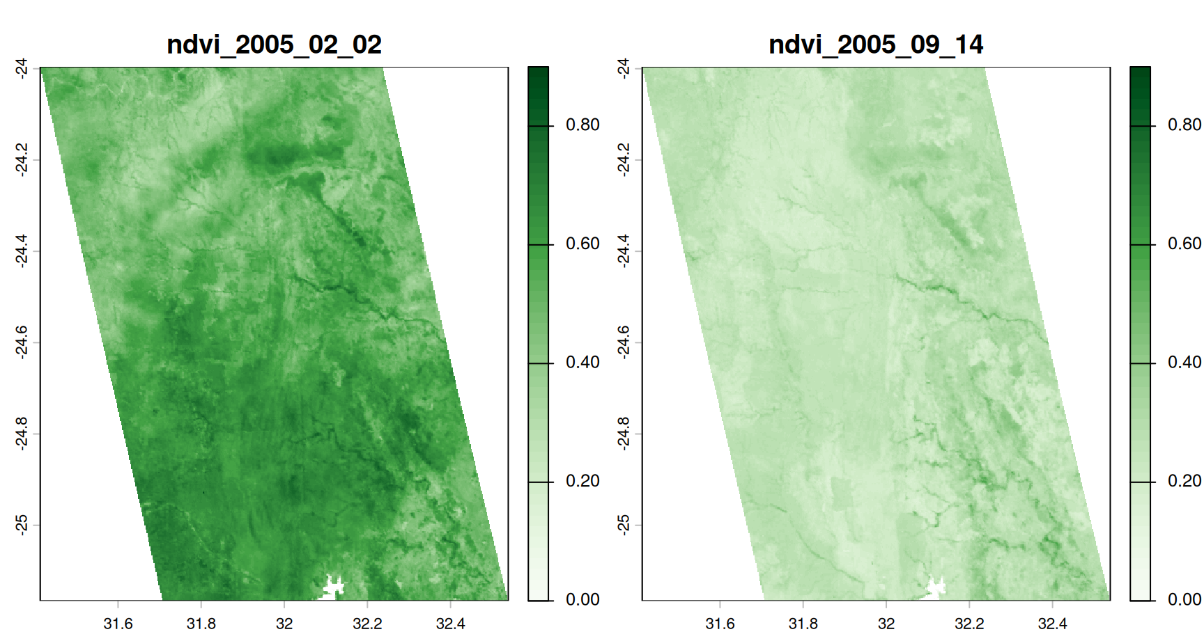

Your turn

4a. What is the resolution in metres? What CRS is it in? 4b. Extract both NDVI layers at every buffalo fix.

Solution

crs(ndvi, describe = TRUE)$code
#> [1] "4326"
res(ndvi)
#> [1] 0.002432149 0.002432149
round(res(ndvi) * c(111320 * cos(24.6 * pi / 180), 111320))   # approx metres
#> [1] 246 271

About 230 m east–west and 230 m north–south — MODIS’s 250 m product, delivered here in longitude/latitude.

fixes$ndvi_wet <- terra::extract(ndvi[["ndvi_2005_02_02"]], vect(fixes))[, 2]
fixes$ndvi_dry <- terra::extract(ndvi[["ndvi_2005_09_14"]], vect(fixes))[, 2]

summary(st_drop_geometry(fixes)[, c("ndvi_wet", "ndvi_dry")])
#>     ndvi_wet         ndvi_dry     
#>  Min.   :0.2920   Min.   :0.1570  
#>  1st Qu.:0.4985   1st Qu.:0.2108  
#>  Median :0.5859   Median :0.2391  
#>  Mean   :0.5674   Mean   :0.2401  
#>  3rd Qu.:0.6426   3rd Qu.:0.2656  
#>  Max.   :0.7435   Max.   :0.3927  
#>  NAs    :1        NAs    :1

The same places are far greener in February than in September. Which value belongs to which fix depends on when the fix was taken — Session 3 does that matching properly.

Task 5 — Break it on purpose

Two silent failures worth recognising for the rest of your career.

A bare coordinate matrix has no CRS

ndvi_utm <- project(ndvi, "EPSG:32736")

# Both objects carry a CRS: terra reprojects for you, with a warning
ok <- terra::extract(ndvi_utm[[1]], vect(fixes))
mean(is.na(ok[, 2]))
#> [1] 4.054657e-05

# A bare matrix carries none: degrees are read as metres
bad <- terra::extract(ndvi_utm[[1]], st_coordinates(fixes))
mean(is.na(bad[, 1]))
#> [1] 1

Every value NA, no error, no warning. Keep coordinates in objects that carry their CRS.

`extract(buffer = )` is ignored for points

at_fix   <- terra::extract(ndvi[[1]], vect(fixes))[, 2]
buf_2000 <- terra::extract(ndvi[[1]], vect(fixes), buffer = 2000,
                           fun = mean, na.rm = TRUE)[, 2]
identical(at_fix, buf_2000)
#> [1] TRUE

The “2 km mean” is the at-fix value, unchanged. Build buffer polygons yourself:

buf_poly <- st_buffer(fixes_utm, 2000) |> st_transform(4326) |> vect()
buf_2000 <- terra::extract(ndvi[[1]], buf_poly, fun = mean, na.rm = TRUE)[, 2]

c(sd_at_fix = sd(at_fix, na.rm = TRUE), sd_2km_mean = sd(buf_2000, na.rm = TRUE))
#>   sd_at_fix sd_2km_mean 
#>  0.09203145  0.08682538

The habit

When an argument is supposed to change the answer, check that it did. identical() costs one line.

Note also what smoothing does: the 2 km mean has less variance than the at-fix value. Here the reduction is modest, because savanna greenness varies mostly at scales larger than 2 km; for a patchier covariate it can be large. Either way, smoothing shrinks the contrast between used and available places. The buffer radius is a hypothesis about perception — choose it from biology, not from whichever radius gives the smallest p-value.

Task 6 — Mini-challenge: a map worth publishing

library(ggspatial)

ndvi_df <- as.data.frame(ndvi_utm[["ndvi_2005_02_02"]], xy = TRUE, na.rm = TRUE)
names(ndvi_df)[3] <- "ndvi"

paths <- fixes_utm |>
  group_by(id) |>
  summarise(do_union = FALSE) |>
  st_cast("LINESTRING")

# Frame the map on where the animals are (robust to a stray fix), plus a margin
xy <- st_coordinates(fixes_utm)
lims_x <- quantile(xy[, 1], c(0.001, 0.999)) + c(-4000, 4000)
lims_y <- quantile(xy[, 2], c(0.001, 0.999)) + c(-4000, 4000)

ggplot() +
  geom_raster(data = ndvi_df, aes(x, y, fill = ndvi)) +
  scale_fill_gradientn(colours = hcl.colors(9, "Greens", rev = TRUE),
                       limits = c(0, 0.9), name = "NDVI\nFeb 2005") +
  geom_sf(data = paths, aes(colour = id), linewidth = 0.3, alpha = 0.85) +
  scale_colour_brewer(palette = "Dark2", name = NULL) +
  annotation_scale(location = "bl", width_hint = 0.25) +
  annotation_north_arrow(location = "tr", style = north_arrow_minimal()) +
  coord_sf(crs = 32736, xlim = lims_x, ylim = lims_y, expand = FALSE) +
  labs(title = "African buffalo in Kruger National Park",
       subtitle = "GPS tracks over wet-season greenness",
       caption = "Tracks: Movebank (Getz et al.). NDVI: MODIS MOD13Q1, 2 Feb 2005.") +
  theme_minimal(base_size = 12) +
  theme(axis.title = element_blank(), legend.position = "right")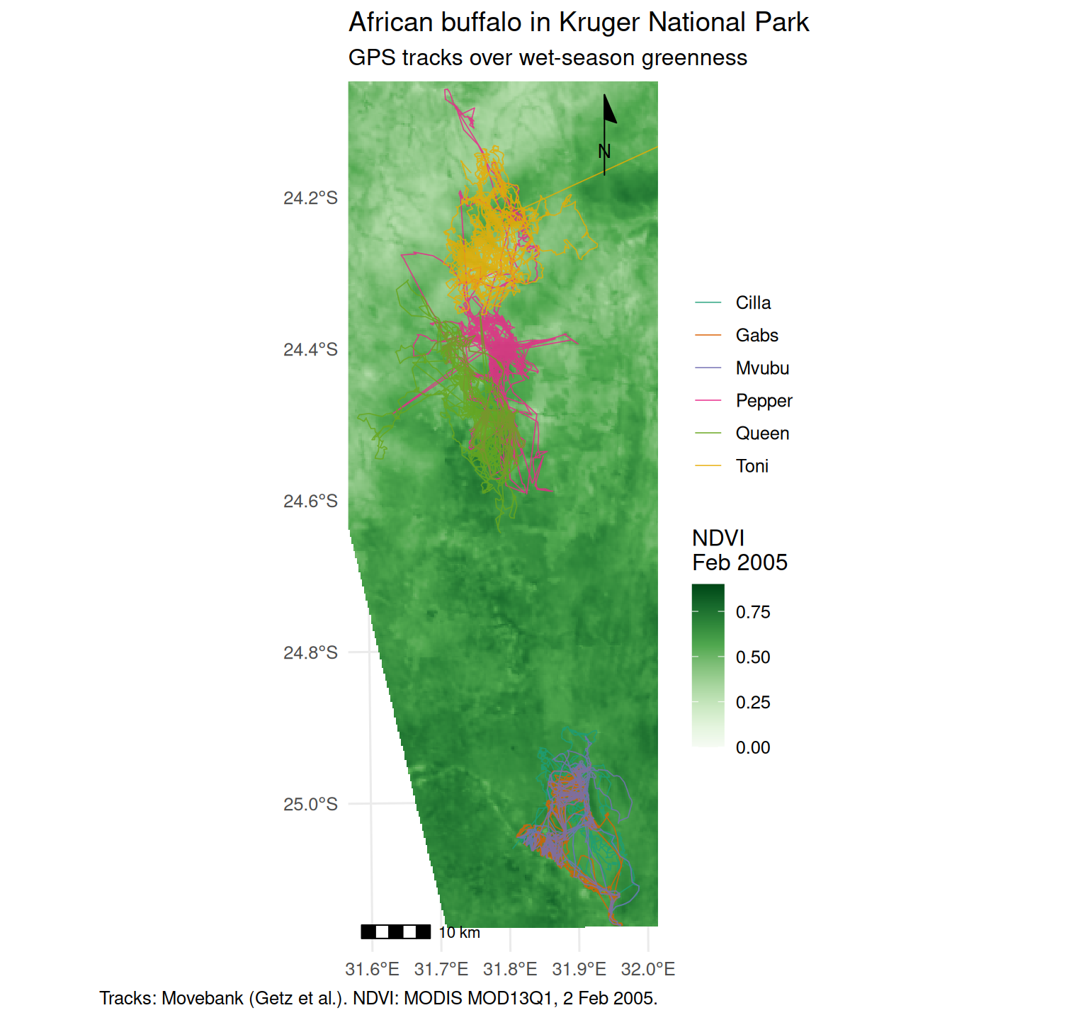

Look at Toni’s track

One straight line leaves the frame towards the north-east. That is a single corrupt fix more than 60 km away — the buffalo did not go there and back in an hour. A good map shows you problems in the data before any model does; Session 3 removes this fix properly.

To hand in

Your own version of this map, as a PNG at print resolution (ggsave("map.png", width = 17, height = 15, units = "cm", dpi = 300)), plus the .qmd that makes it. It must have: a projected CRS, a scale bar, a legend with units, a caption crediting the data, and colours that survive greyscale printing. Choose a different layer or animal from the one above.

Self-check

st_crs(x) <- 32736 on an object whose coordinates are longitude/latitude. What have you done?

Reprojected the data to UTM 36S
Mislabelled the data — the numbers are unchanged but now claimed to be metres
Nothing; sf ignores invalid assignments
Produced an error

Assigning a CRS only writes a label. 31.8 and −24.5 are now read as metres from the UTM 36S origin — a point off West Africa. It fails silently, which is what makes it dangerous. st_transform() changes coordinates.

You st_join() 20,000 fixes to a habitat layer and get back 20,412 rows. Why?

st_join() duplicates the last row
Some fixes fall in more than one polygon (overlaps, or exactly on a shared boundary)
The CRSs differ
It is a bug in sf

st_join() is a spatial left join: one output row for every match. A point on a shared boundary, or inside overlapping polygons, matches twice. Always compare row counts before and after a join, and use largest = TRUE (for polygons) or clean the polygon layer so it tiles without overlaps.

Before Session 3

Make sure library(amt) and library(adehabitatLT) both load.

Task 1 — From data frame to sf

Your turn

Task 2 — Reproject, and measure one distance three ways

Task 3 — Vector verbs: buffer, join, intersect

st_join() — which polygon is each fix in?

st_buffer() and st_intersection() — what is around the animal?

Your turn

Task 4 — Rasters with terra: NDVI

Your turn

Task 5 — Break it on purpose

A bare coordinate matrix has no CRS

extract(buffer = ) is ignored for points

Task 6 — Mini-challenge: a map worth publishing

Self-check

Before Session 3

Task 1 — From data frame to `sf`

`st_join()` — which polygon is each fix in?

`st_buffer()` and `st_intersection()` — what is around the animal?

Task 4 — Rasters with `terra`: NDVI

`extract(buffer = )` is ignored for points