Practical 3 — From fixes to trajectories

Session 3 · Data cleaning, bursts, resampling

Modified

September 30, 2026

Goals. Build a trajectory in amt and in adehabitatLT; clean it and count what you remove; quantify and visualise sampling irregularity; resample by selection and by interpolation and see the difference; label day and night; attach NDVI matched to the time of each fix.

Time: ~75 minutes. Packages: amt, adehabitatLT, terra, dplyr, tidyr, lubridate, ggplot2.

library(amt)
library(adehabitatLT)
library(terra)
library(dplyr)
library(tidyr)
library(lubridate)
library(ggplot2)

Task 1 — Build a track

raw <- read.csv("data/buffalo_kruger.csv.gz") |>
  transmute(
    id = individual.local.identifier,
    t  = as.POSIXct(timestamp, tz = "UTC"),
    x  = location.long,
    y  = location.lat
  )

nrow(raw)
#> [1] 28410

Now clean, counting every step. This block is the template for every dataset you will ever handle.

n0 <- nrow(raw)

clean <- raw |> filter(!is.na(x), !is.na(y))
n1 <- nrow(clean)

clean <- clean |> filter(!(x == 0 & y == 0))
n2 <- nrow(clean)

clean <- clean |> distinct(id, t, .keep_all = TRUE)
n3 <- nrow(clean)

data.frame(
  step = c("raw", "drop missing coords", "drop (0,0)", "drop duplicate id+time"),
  rows = c(n0, n1, n2, n3),
  removed = c(NA, n0 - n1, n1 - n2, n2 - n3)
)
#>                     step  rows removed
#> 1                    raw 28410      NA
#> 2    drop missing coords 28410       0
#> 3             drop (0,0) 28410       0
#> 4 drop duplicate id+time 24663    3747

Always produce this table

It goes in your methods section, and it is the first thing a reviewer — or a future you — will want. “We removed 3,747 duplicated records (13.2%)” is a sentence you can defend. “We cleaned the data” is not.

trk <- make_track(clean, x, y, t, id = id, crs = 4326) |>
  transform_coords(crs_to = 32736)

trk
#> # A tibble: 24,663 × 4
#>         x_       y_ t_                  id   
#>  *   <dbl>    <dbl> <dttm>              <chr>
#>  1 375051. 7285726. 2005-02-17 05:05:00 Queen
#>  2 374851. 7285502. 2005-02-17 06:08:00 Queen
#>  3 374527. 7284538. 2005-02-17 07:05:00 Queen
#>  4 374492. 7284644. 2005-02-17 08:05:00 Queen
#>  5 374392. 7284667. 2005-02-17 09:05:00 Queen
#>  6 374378. 7284668. 2005-02-17 10:05:00 Queen
#>  7 374422. 7284666. 2005-02-17 11:05:00 Queen
#>  8 374430. 7284663. 2005-02-17 12:05:00 Queen
#>  9 374426. 7284662. 2005-02-17 13:05:00 Queen
#> 10 374733. 7284627. 2005-02-17 14:05:00 Queen
#> # ℹ 24,653 more rows

Your turn

1a. What class is trk? What are its columns called? 1b. Confirm the coordinates are now metres.

Solution

class(trk)
#> [1] "track_xyt"  "track_xy"   "tbl_df"     "tbl"        "data.frame"
names(trk)
#> [1] "x_" "y_" "t_" "id"
summary(trk$x_)
#>    Min. 1st Qu.  Median    Mean 3rd Qu.    Max. 
#>  356761  375417  379046  380566  386182  434568

track_xyt — a tibble with x_, y_, t_ plus the columns you carried along. The coordinates are now six-figure eastings and seven-figure northings: UTM 36S metres.

Task 1b — The same trajectory as an `ltraj`

adehabitatLT stores a trajectory as a list of bursts, with the step descriptors already computed.

cilla <- trk |> filter(id == "Cilla")

ltr <- as.ltraj(xy = as.data.frame(cilla[, c("x_", "y_")]),
                date = cilla$t_, id = "Cilla")
ltr
#> 
#> *********** List of class ltraj ***********
#> 
#> Type of the traject: Type II (time recorded)
#> * Time zone: UTC *
#> Irregular traject. Variable time lag between two locs
#> 
#> Characteristics of the bursts:
#>      id burst nb.reloc NAs          date.begin            date.end
#> 1 Cilla Cilla     3528   0 2005-07-14 04:35:00 2005-12-07 22:16:00
#> 
#> 
#>  infolocs provided. The following variables are available:
#> [1] "pkey"

head(ld(ltr)[, c("date", "dist", "dt", "R2n", "abs.angle", "rel.angle")])
#>                  date       dist   dt       R2n  abs.angle rel.angle
#> 1 2005-07-14 04:35:00 13386.3440 3600         0  0.9006608        NA
#> 2 2005-07-14 05:35:00  3943.3528 7200 179194206  2.3910145 1.4903537
#> 3 2005-07-14 07:35:00   817.9605 3540 203227744 -2.1217678 1.7704030
#> 4 2005-07-14 08:34:00   593.9637 3660 180873970 -1.2480422 0.8737256
#> 5 2005-07-14 09:35:00   814.8749 3600 169047094  1.2209400 2.4689822
#> 6 2005-07-14 10:35:00  2097.6577 3540 190861649  2.3937138 1.1727738

dist is step length (m), dt the interval (s), R2n the squared distance from the first fix (we use it in Session 4), and rel.angle the turning angle.

Your turn

1c. Compute step lengths and turning angles with amt and check they agree with the ltraj columns.

Solution

st_cilla <- cilla |> steps()
c(amt_median_sl = median(st_cilla$sl_),
  ltraj_median_dist = median(ld(ltr)$dist, na.rm = TRUE))
#>     amt_median_sl ltraj_median_dist 
#>          149.4087          149.4087

# amt's ta_ and adehabitat's rel.angle are the same quantity
a <- st_cilla$ta_[-1]
b <- ld(ltr)$rel.angle[2:nrow(st_cilla)]
both <- !is.na(a) & !is.na(b)

naive    <- max(abs(a[both] - b[both]))                       # plain subtraction
circular <- max(abs(atan2(sin(a[both] - b[both]),             # difference on
                          cos(a[both] - b[both]))))           # the circle
c(compared = sum(both), naive_max_diff = naive, circular_max_diff = circular,
  NA_in_amt = sum(is.na(a)), NA_in_adehabitat = sum(is.na(b)))
#>          compared    naive_max_diff circular_max_diff         NA_in_amt 
#>      3.516000e+03      6.283185e+00      8.881784e-16      1.000000e+01 
#>  NA_in_adehabitat 
#>      5.000000e+00

Two lessons in one table.

Angles are circular. Plain subtraction reports a maximum difference of exactly 2π — one package wrote a U-turn as +π, the other as −π, which are the same direction. Measured on the circle the difference is zero. Never compare, average or subtract angles as ordinary numbers.

Undefined angles. The packages disagree on how many turns to leave undefined around zero-length steps: a step of 0 m has no direction, so the turn into or out of it cannot be computed. amt blanks more of them than adehabitatLT does. Worth knowing before you compare turning-angle distributions across packages.

Otherwise: same numbers, different containers. Use whichever the next analysis needs: ltraj for first-passage time and Brownian bridges (Sessions 4 and 6), amt for resampling and step selection.

Task 2 — Sampling rate

trk |>
  summarize_sampling_rate_many(cols = "id", time_unit = "hour") |>
  mutate(across(where(is.numeric), \(z) round(z, 2)))
#> # A tibble: 6 × 10
#>   id       min    q1 median  mean    q3   max    sd     n unit 
#>   <chr>  <dbl> <dbl>  <dbl> <dbl> <dbl> <dbl> <dbl> <dbl> <chr>
#> 1 Queen   0.03     1      1  2.45  1    2523. 50.5   4544 hour 
#> 2 Gabs    0.03     1      1  1.22  1     723. 12.0   3669 hour 
#> 3 Cilla   0.05     1      1  1     1       2   0.05  3527 hour 
#> 4 Mvubu   0.03     1      1  0.99  1       9   0.2   2571 hour 
#> 5 Toni    0.08     1      1  1.01  1      17   0.26  5776 hour 
#> 6 Pepper  0.02     1      1  2.47  1.98 1603. 24.6   4570 hour

Your turn

2a. What is the programmed fix interval? 2b. Why is the mean so much larger than the median? 2c. Which individual has the worst gap, and how long is it in days?

Solution

The median is 1 hour for every animal — that is the schedule. The mean is inflated by a handful of enormous gaps:

gaps <- trk |>
  group_by(id) |>
  arrange(t_, .by_group = TRUE) |>
  mutate(dt_h = as.numeric(difftime(t_, lag(t_), units = "hours"))) |>
  ungroup()

gaps |>
  group_by(id) |>
  summarise(
    median_dt = median(dt_h, na.rm = TRUE),
    mean_dt   = round(mean(dt_h, na.rm = TRUE), 1),
    max_gap_days = round(max(dt_h, na.rm = TRUE) / 24, 1),
    gaps_over_1d = sum(dt_h > 24, na.rm = TRUE),
    .groups = "drop"
  )
#> # A tibble: 6 × 5
#>   id     median_dt mean_dt max_gap_days gaps_over_1d
#>   <chr>      <dbl>   <dbl>        <dbl>        <int>
#> 1 Cilla          1     1            0.1            0
#> 2 Gabs           1     1.2         30.1            2
#> 3 Mvubu          1     1            0.4            0
#> 4 Pepper         1     2.5         66.8           40
#> 5 Queen          1     2.4        105.             9
#> 6 Toni           1     1            0.7            0

Always report the median. A mean sampling interval is a summary of your collar failures, not of your sampling design.

Task 3 — Hunt the speed outliers

First, look. Then delete.

steps_raw <- trk |>
  group_by(id) |>
  arrange(t_, .by_group = TRUE) |>
  mutate(
    dt_h = as.numeric(difftime(t_, lag(t_), units = "hours")),
    dist_m = sqrt((x_ - lag(x_))^2 + (y_ - lag(y_))^2),
    speed_kmh = (dist_m / 1000) / dt_h
  ) |>
  ungroup() |>
  filter(!is.na(speed_kmh))

summary(steps_raw$speed_kmh)
#>     Min.  1st Qu.   Median     Mean  3rd Qu.     Max. 
#>  0.00000  0.03129  0.15101  0.29545  0.38204 63.10252
sum(steps_raw$speed_kmh > 15)
#> [1] 4

Your turn

3a. Look at the fastest steps. Are they long or are they brief?

Solution

steps_raw |>
  slice_max(speed_kmh, n = 10) |>
  transmute(id, t_, dt_min = round(dt_h * 60, 1),
            dist_m = round(dist_m), speed_kmh = round(speed_kmh))
#> # A tibble: 10 × 5
#>    id     t_                  dt_min dist_m speed_kmh
#>  * <chr>  <dttm>               <dbl>  <dbl>     <dbl>
#>  1 Toni   2006-04-20 19:10:00     60  63103        63
#>  2 Toni   2006-04-20 18:10:00     61  63067        62
#>  3 Pepper 2006-05-24 05:06:00     60  17379        17
#>  4 Pepper 2006-05-24 06:07:00     61  16804        17
#>  5 Cilla  2005-07-14 05:35:00     60  13386        13
#>  6 Queen  2005-09-15 07:41:00     70  11783        10
#>  7 Pepper 2006-05-23 15:06:00     60   9898        10
#>  8 Queen  2006-05-26 04:16:00      2    314         9
#>  9 Pepper 2005-10-21 23:02:00      3    255         5
#> 10 Queen  2005-03-26 00:00:00     60   4728         5

The worst offenders have tiny time gaps, not large distances — a couple of hundred metres over a minute or two. These are near-duplicate transmissions that survived the exact-duplicate filter.

Confirm it across all the fast steps:

fast <- steps_raw |> filter(speed_kmh > 15)
summary(fast$dt_h * 60)     # minutes
#>    Min. 1st Qu.  Median    Mean 3rd Qu.    Max. 
#>    60.0    60.0    60.5    60.5    61.0    61.0
summary(fast$dist_m)        # metres
#>    Min. 1st Qu.  Median    Mean 3rd Qu.    Max. 
#>   16804   17235   40223   40088   63076   63103

plot(steps_raw$dt_h * 60, steps_raw$speed_kmh, log = "xy",
     pch = 16, cex = 0.25, col = adjustcolor("#1f6f78", 0.25),
     xlab = "Time gap (minutes, log)", ylab = "Speed km/h (log)",
     main = "Fast steps are short-interval steps")
abline(h = 15, col = "firebrick", lty = 2, lwd = 2)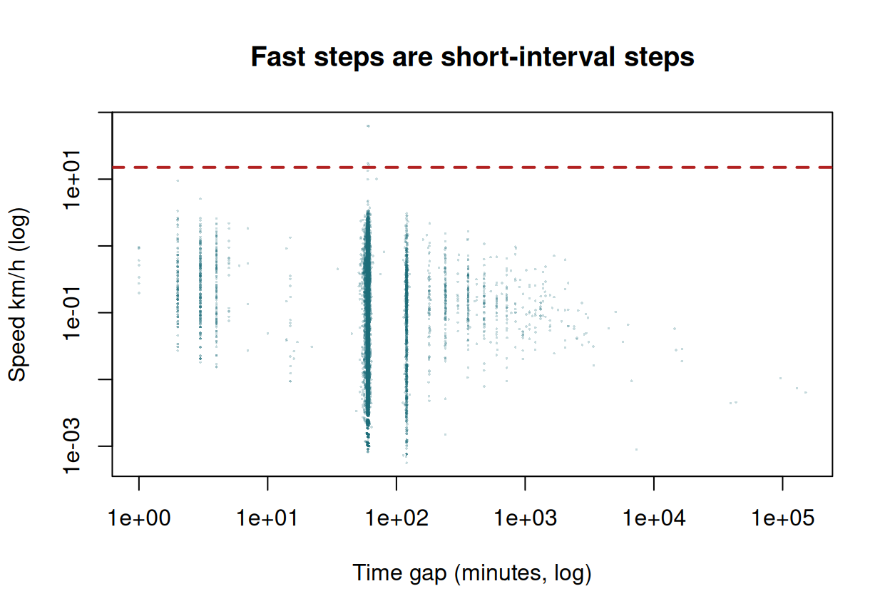

The diagonal edge is the signature: apparent speed is bounded by (GPS error)/dt, so as dt shrinks, apparent speed explodes. This is a time problem masquerading as a speed problem — and deleting the “fast” fixes would remove perfectly good locations.

The correct remedy is to resample onto a regular grid, which is Task 4.

Task 4 — Resample into bursts

This is where almost everyone writes a silent bug. Try the obvious thing first.

# The "obvious" pipeline — grouped by individual
naive <- trk |>
  group_by(id) |>
  track_resample(rate = hours(1), tolerance = minutes(10)) |>
  filter_min_n_burst(min_n = 3) |>
  ungroup()

nrow(trk)
#> [1] 24663
nrow(naive)
#> [1] 10395
naive |> count(id, name = "kept")
#> # A tibble: 6 × 2
#>   id      kept
#>   <chr>  <int>
#> 1 Cilla   2731
#> 2 Gabs    1921
#> 3 Mvubu    166
#> 4 Pepper   644
#> 5 Queen   1741
#> 6 Toni    3192

track_resample() does not respect group_by()

Look at the per-animal counts. Mvubu goes from 2,572 fixes to a couple of hundred — but Mvubu’s data are fine: 98.8% of that animal’s intervals are within 10 minutes of one hour.

track_resample() walks the rows in time order and builds one grid across everything you hand it. With six animals interleaved, fixes from animal B fall between the grid points of animal A, and most of the track is discarded. No error. No warning. Just a much smaller dataset.

The documented amt idiom is to split, resample each animal separately, and recombine:

library(tidyr)

trk_hr <- trk |>
  nest(data = -id) |>
  mutate(data = lapply(data, \(d) {
    d |>
      track_resample(rate = hours(1), tolerance = minutes(10)) |>
      filter_min_n_burst(min_n = 3)
  })) |>
  unnest(cols = data)

nrow(trk_hr)
#> [1] 22828

trk |> count(id, name = "before") |>
  left_join(naive   |> count(id, name = "grouped_WRONG"), by = "id") |>
  left_join(trk_hr  |> count(id, name = "nested_right"), by = "id") |>
  mutate(pct_kept = round(100 * nested_right / before, 1))
#> # A tibble: 6 × 5
#>   id     before grouped_WRONG nested_right pct_kept
#> * <chr>   <int>         <int>        <int>    <dbl>
#> 1 Cilla    3528          2731         3518     99.7
#> 2 Gabs     3670          1921         3562     97.1
#> 3 Mvubu    2572           166         2544     98.9
#> 4 Pepper   4571           644         3086     67.5
#> 5 Queen    4545          1741         4354     95.8
#> 6 Toni     5777          3192         5764     99.8

Now we keep ~93% of the fixes, which is what an hourly schedule with occasional failures should give.

Your turn

4a. Recompute speeds on the correctly resampled track. Did the problem go away? 4b. What happens if you set tolerance = minutes(1)?

Solution

st <- trk_hr |> steps_by_burst()

summary(as.numeric(st$dt_, units = "mins"))
#>    Min. 1st Qu.  Median    Mean 3rd Qu.    Max. 
#>      54      60      60      60      60      70

sp <- (st$sl_ / 1000) / as.numeric(st$dt_, units = "hours")
round(quantile(sp, c(0.5, 0.9, 0.99, 0.999, 1)), 2)
#>   50%   90%   99% 99.9%  100% 
#>  0.15  0.73  1.93  3.05 63.10
sum(sp > 15)
#> [1] 4

Every step now spans 50–70 minutes, and the time-artefact speeds are gone: the median is a few hundred metres per hour, which is what a buffalo does.

But a handful of steps remain absurdly fast. These are different animals entirely — look at them:

st[sp > 15, c("t1_", "sl_", "dt_")] |> head(5)
#> # A tibble: 4 × 3
#>   t1_                    sl_ dt_    
#> * <dttm>               <dbl> <drtn> 
#> 1 2006-04-20 17:09:00 63067. 61 mins
#> 2 2006-04-20 18:10:00 63103. 60 mins
#> 3 2006-05-24 04:06:00 17379. 60 mins
#> 4 2006-05-24 05:06:00 16804. 61 mins

Sixty-five kilometres in an hour. That is not a short time gap; it is a genuine spatial outlier — a corrupt fix that teleported the animal and back. Now that every step spans the same interval, a fast step really does mean a long distance, and a speed filter finally does what you meant it to do.

plot(as.numeric(st$dt_, units = "mins"), sp, log = "y", pch = 16, cex = 0.3,
     col = adjustcolor("#1f6f78", 0.3),
     xlab = "Step duration (minutes)", ylab = "Speed km/h (log)",
     main = "After resampling: fast = far, not brief")
abline(h = 15, col = "firebrick", lty = 2, lwd = 2)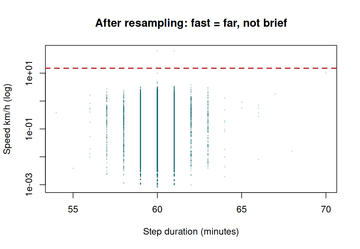

Compare this with the plot in Task 3: the diagonal artefact edge has gone, and what is left above the line is a small, isolated cluster of real errors.

tight <- trk |>
  nest(data = -id) |>
  mutate(data = lapply(data, \(d) d |>
    track_resample(rate = hours(1), tolerance = minutes(1)) |>
    filter_min_n_burst(min_n = 3))) |>
  unnest(cols = data)

c(tolerance_10min = nrow(trk_hr), tolerance_1min = nrow(tight))
#> tolerance_10min  tolerance_1min 
#>           22828           21903

A tight tolerance discards fixes that arrived a few minutes late — real data you would rather keep. A loose one lets “hourly” steps range from 40 to 80 minutes, weakening every step-length comparison. 5–10% of the interval is a reasonable compromise; state whichever you chose.

Task 5 — Now try the bats

bat <- read.csv("data/bat_safi.csv.gz") |>
  transmute(id = individual.local.identifier,
            t  = as.POSIXct(timestamp, tz = "UTC"),
            x  = location.long, y = location.lat) |>
  filter(!is.na(x), !is.na(y)) |>
  distinct(id, t, .keep_all = TRUE)

bat_trk <- make_track(bat, x, y, t, id = id, crs = 4326) |>
  transform_coords(crs_to = 32632)     # UTM 32N, Switzerland

bat_trk |>
  summarize_sampling_rate_many(cols = "id", time_unit = "min") |>
  mutate(across(where(is.numeric), \(z) round(z, 1))) |>
  head(8)
#> # A tibble: 8 × 10
#>      id   min    q1 median  mean    q3   max    sd     n unit 
#>   <dbl> <dbl> <dbl>  <dbl> <dbl> <dbl> <dbl> <dbl> <dbl> <chr>
#> 1    21   1.7   5.2      9 116.   18.8 1605   354.   126 min  
#> 2   289   0.1   6        9 127.   18   1623   372.   161 min  
#> 3   127   0.1   7.2     10 114.   21.8 1448.  344.   114 min  
#> 4   570   0.1   7       11 150.   26   1445.  394.    95 min  
#> 5   146  10    10       10  89.7  12.5 1260   299.    32 min  
#> 6    42  10    10       10 110    10   1310   345.    26 min  
#> 7   168   8     8        8  88.9  10   2764   372.   164 min  
#> 8   495   8     8        8 142.   10   4246   591.   103 min

Your turn

5a. Try to resample the bats to a regular 15-minute interval. What survives? 5b. What would you do instead?

Solution

bat_15 <- bat_trk |>
  nest(data = -id) |>
  mutate(data = lapply(data, \(d) d |>
    track_resample(rate = minutes(15), tolerance = minutes(5)) |>
    filter_min_n_burst(min_n = 3))) |>
  unnest(cols = data)

c(before = nrow(bat_trk), after = nrow(bat_15))
#> before  after 
#>   1740    802

bursts <- bat_15 |> count(id, burst_)
c(n_bursts = nrow(bursts), median_length = median(bursts$n), max_length = max(bursts$n))
#>      n_bursts median_length    max_length 
#>           165             4            13
table(bursts$n)
#> 
#>  3  4  5  6  7  8  9 10 11 13 
#> 57 34 26 20  8  7  5  4  2  2

Fewer than half the fixes survive — but the real problem is the shape of what is left. The 802 surviving fixes shatter into 165 bursts with a median length of 4, i.e. three steps each. There is no programmed schedule to recover: fixes arrived whenever a field worker obtained a bearing.

A hidden Markov model (Session 8) estimates transition probabilities between behavioural states. With bursts of three steps, there is almost nothing to transition — you would be asking the model to learn the dynamics of a process from fragments shorter than the process itself.

lags <- bat_trk |>
  group_by(id) |>
  arrange(t_, .by_group = TRUE) |>
  mutate(dt_min = as.numeric(difftime(t_, lag(t_), units = "mins"))) |>
  ungroup() |> filter(!is.na(dt_min), dt_min > 0)

hist(log10(lags$dt_min), breaks = 40, col = "#1f6f78", border = "white",
     xlab = "log10 interval (minutes)", main = "Bat sampling intervals span five orders of magnitude")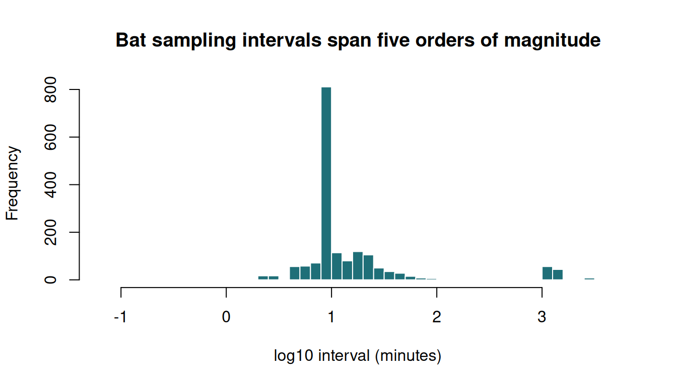

What to do instead. Not: force a regular grid and pretend. The honest options are

restrict to the questions these data can answer — which sites were used, broad home-range extent, night-time activity periods;
use methods that tolerate irregular sampling, i.e. continuous-time models (ctmm) rather than discrete-step models;
treat each night as a separate short burst and analyse only within-night movement.

Recognising which of your datasets is a “buffalo” and which is a “bat” is one of the more valuable things you will take from this course.

Task 6 — Interpolation is not resampling

adehabitatLT::redisltraj() also produces a regular hourly series — by inventing positions.

cilla_ltr <- as.ltraj(xy = as.data.frame(cilla[, c("x_", "y_")]),
                      date = cilla$t_, id = "Cilla")
interp <- redisltraj(cilla_ltr, 3600, type = "time")

selected <- trk_hr |> filter(id == "Cilla")

c(original_fixes = nrow(cilla),
  selected_by_track_resample = nrow(selected),
  produced_by_redisltraj = nrow(ld(interp)))
#>             original_fixes selected_by_track_resample 
#>                       3528                       3518 
#>     produced_by_redisltraj 
#>                       3522

Your turn

6a. How many of the interpolated positions coincide with a real fix? 6b. What would interpolated positions do to a step-length distribution?

Solution

real_times <- cilla$t_
interp_times <- ld(interp)$date
sum(interp_times %in% real_times)
#> [1] 30
length(interp_times)
#> [1] 3522

Almost none of the “hourly” positions is an observation: redisltraj() walks along the straight lines between fixes and places a point every 3,600 seconds. Every one of those points assumes the animal moved at constant speed in a straight line between fixes.

Consequences: step lengths across a gap become artificially uniform, turning angles on interpolated stretches become exactly zero, and any model fitted to them sees a smooth, persistent animal that never existed. Use interpolation for display, never as data — or use a model that interpolates with uncertainty (ctmm, crawl), which is what Sessions 6 and 8 do.

Task 7 — Day or night?

Many behaviours are diel. time_of_day() labels each fix from the sun’s position at that place and time.

cilla_tod <- selected |>
  time_of_day()

cilla_steps <- cilla_tod |>
  steps_by_burst(keep_cols = "start")

cilla_steps |>
  group_by(tod_) |>
  summarise(steps = n(), median_sl_m = round(median(sl_)),
            mean_sl_m = round(mean(sl_)))
#> # A tibble: 2 × 4
#>   tod_  steps median_sl_m mean_sl_m
#>   <fct> <int>       <dbl>     <dbl>
#> 1 day    1801         221       347
#> 2 night  1714         104       218

What this shows

Buffalo move further per hour by day than by night — a diel pattern you must account for before interpreting anything else about their movement. In Session 8 we let the probability of switching behavioural state depend on the time of day.

Task 8 — NDVI matched to the time of each fix

The NDVI raster from Session 2 has two layers, a wet-season composite (2 Feb 2005) and a dry-season one (14 Sep 2005). Tell terra when each was taken, then let amt give every fix the value of the composite closest in time.

ndvi <- project(rast("data/kruger_ndvi_2005.tif"), "EPSG:32736")
time(ndvi) <- as.POSIXct(c("2005-02-02", "2005-09-14"), tz = "UTC")
ndvi
#> class       : SpatRaster
#> size        : 504, 445, 2  (nrow, ncol, nlyr)
#> resolution  : 258.5037, 258.5037  (x, y)
#> extent      : 338541.4, 453575.6, 7215872, 7346158  (xmin, xmax, ymin, ymax)
#> coord. ref. : WGS 84 / UTM zone 36S (EPSG:32736)
#> source(s)   : memory
#> names       : ndvi_2005_02_02, ndvi_2005_09_14
#> min values  :       -0.196056,       -0.198263
#> max values  :        0.804637,        0.583936
#> time        : 2005-02-02 00:00:00zUTC to 2005-09-14 00:00:00zUTC (2 steps)

queen <- trk |> filter(id == "Queen", year(t_) == 2005)

queen_ndvi <- queen |>
  extract_covariates_var_time(ndvi, when = "any", max_time = days(45),
                              name_covar = "ndvi")

queen_ndvi |>
  mutate(month = month(t_, label = TRUE)) |>
  group_by(month) |>
  summarise(fixes = n(), with_ndvi = sum(!is.na(ndvi)),
            mean_ndvi = round(mean(ndvi, na.rm = TRUE), 3))
#> # A tibble: 9 × 4
#>   month fixes with_ndvi mean_ndvi
#>   <ord> <int>     <int>     <dbl>
#> 1 Feb     285       285     0.59 
#> 2 Mar     751       438     0.607
#> 3 Apr     646         0   NaN    
#> 4 May      73         0   NaN    
#> 5 Jun       1         0   NaN    
#> 6 Sep     319       319     0.252
#> 7 Oct     676       604     0.252
#> 8 Nov     719         0   NaN    
#> 9 Dec     737         0   NaN

Your turn

8a. Why are most months NA? 8b. What would you need to annotate the whole year?

Solution

With max_time = days(45), a fix is annotated only if a composite exists within 45 days of it. We have two composites, so only February–March and September–October are covered. Everything else is honestly NA — far better than silently assigning February’s greenness to a July fix.

To annotate the whole year you need the full series: MOD13Q1 produces a composite every 16 days, 23 per year. The same MODISTools call that built this file fetches them all — it just takes longer:

library(MODISTools)
ndvi_ts <- mt_subset(product = "MOD13Q1", band = "250m_16_days_NDVI",
                     lat = -24.58, lon = 31.97, km_lr = 45, km_ab = 70,
                     start = "2005-01-01", end = "2006-12-31")
ndvi_ts <- mt_to_terra(ndvi_ts, reproject = TRUE)   # already scaled to NDVI units

Or upload the track to Movebank’s Env-DATA, which does the matching and the temporal interpolation for you. Either way, check the result with summary(): NDVI must lie between −1 and 1. If you see values in the thousands, the scale factor was not applied; if you see values a thousand times too small, it was applied twice.

To hand in

Weekly submission

For one buffalo: (1) the cleaning table from Task 1; (2) a histogram of sampling intervals on a log scale; (3) two sentences stating which of the analyses in the slides’ “who tolerates irregular sampling” table you could apply to this animal without resampling, and why.

Self-check

Which cleaning order is correct?

Speed filter → remove duplicates → resample
Remove duplicates → resample to a regular rate → inspect remaining outliers
Resample → remove duplicates → speed filter
The order does not matter

Duplicates and near-duplicates create tiny time gaps, and tiny time gaps create enormous apparent speeds. Filter on speed first and you delete good fixes for a fault that belongs to their neighbours.

Remove duplicates, then resample so that every step spans a comparable interval, and then look at what is still implausible. By that point, a genuinely fast step really is a long distance.

You pipe six animals into group_by(id) |> track_resample(rate = hours(1)) and keep 42% of your fixes. The same animals resampled one at a time keep 93%. Why?

track_resample() ignores group_by() and builds one time grid across all animals
group_by() removed the duplicate timestamps
The tolerance was too tight
42% is correct; the per-animal version double-counts

track_resample() walks the rows in time order and lays a single regular grid over whatever you give it. Hand it six interleaved animals and most fixes fall between grid points set by some other individual, so they are dropped.

It fails silently — no error, no warning, just a smaller dataset — which is what makes it dangerous. Use the nest() / lapply() / unnest() idiom so each animal gets its own grid.

The general lesson: not every function respects dplyr grouping. When a step drops far more data than you expected, check the per-group counts before you accept the result.

Before Session 4

vignette("p1_basics", package = "amt")
Read Powell & Mitchell (2012), What is a home range? — it is short and it will change how you read the next twenty papers.

Task 1 — Build a track

Your turn

Task 1b — The same trajectory as an ltraj

Your turn

Task 2 — Sampling rate

Your turn

Task 3 — Hunt the speed outliers

Your turn

Task 4 — Resample into bursts

Your turn

Task 5 — Now try the bats

Your turn

Task 6 — Interpolation is not resampling

Your turn

Task 7 — Day or night?

Task 8 — NDVI matched to the time of each fix

Your turn

To hand in

Self-check

Before Session 4

Task 1b — The same trajectory as an `ltraj`