From fixes to trajectories

Session 3 — Data cleaning, bursts, resampling

Giuliano Colosimo

University of Rome Tor Vergata

2026-10-06

Today

Internal state Motion capacity Navigation capacity External factors Movement path

We turn a table of fixes into a path we can defend, and attach the environment to it — in space and in time.

Where we are going

Position data are not path data: what a step and a turning angle really are
Location error, and why you cannot just connect the dots
Cleaning: duplicates, impossible locations, speed outliers
Bursts, gaps and truncation; resampling to a regular grid
Which analyses tolerate irregular sampling, and which do not
Annotating a trajectory with environment matched in time

80% of a movement analysis is getting the data into a defensible state. Today is that 80%.

1 · Positions are not paths

What a GPS track actually is

A set of point estimates, each with an error, at irregular moments
Between two fixes the animal went somewhere; the straight line is an assumption, not an observation
Interpolating a position between fixes invents data — useful for plotting, dangerous for inference
Every derived quantity — step length, speed, turning angle — inherits both the sampling interval and the location error

A track is a sample of a continuous path. Treat every line you draw between fixes as a hypothesis.

The step

Two consecutive fixes define a step.

Step length \(s_t = \lVert \mathbf{x}_{t+1} - \mathbf{x}_t \rVert\)
Absolute direction \(\phi_t = \operatorname{atan2}(\Delta y, \Delta x)\)
Turning angle \(\theta_t = \phi_t - \phi_{t-1}\), wrapped to \((-\pi, \pi]\)
Speed \(v_t = s_t / \Delta t\)

A turning angle needs three fixes. A step needs two. That is why filter_min_n_burst(min_n = 3) exists.

Turning angles are circular data: −179° and +179° are 2° apart, not 358°. Never take an arithmetic mean of angles.

Steps and turns of a real buffalo

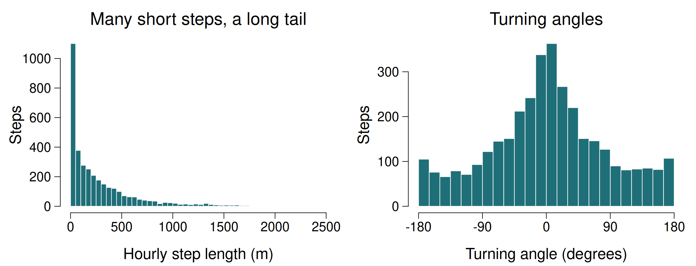
Cilla, hourly steps. Short steps dominate; turning angles concentrate near 0° (keep going). The bars at −180° and +180° are the same reversal, split in two by the axis.

Location error: why you cannot connect the dots

A 15 m error on each fix is negligible on a 1 km step, and dominates a 20 m step
For short steps the direction is mostly noise, so turning angles look random exactly when the animal is resting
A single bad fix creates a spike: an impossible step out and back
Error is not independent white noise: it is correlated in time and worse in closed habitat

Resting animals look like they are wandering at random, and spikes look like sprints. Neither is behaviour. Both reach your models unless you look first.

What error looks like

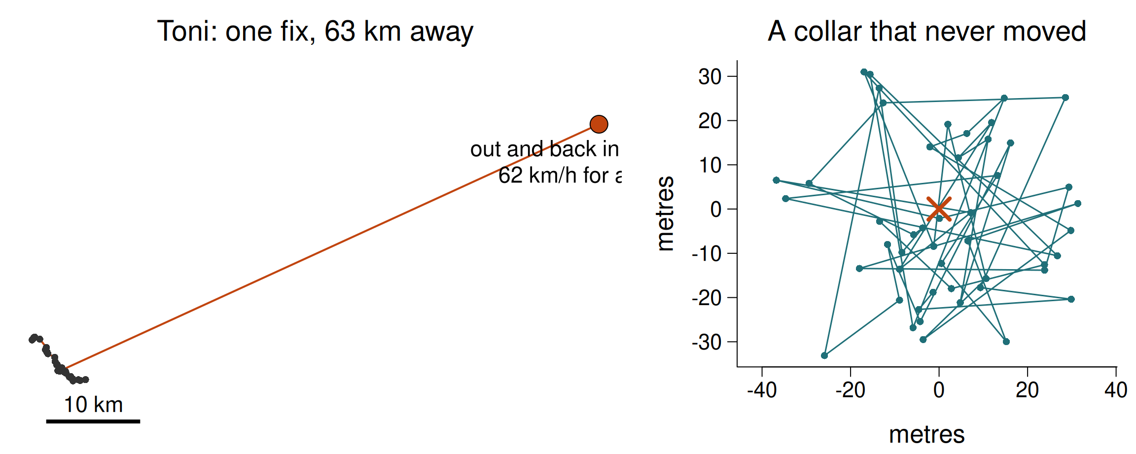
Left: real data, 24 hours either side of a corrupt fix. Right: simulated — 48 hourly fixes of a motionless collar with 15 m error. It “walks” 1 km a day and turns at random.

2 · Getting data

Movebank in R

library(move2)

# Interactive login, stored in your keyring
movebank_store_credentials("your_username")

# What is available?
movebank_download_study_info(license_type = "CC_0")

# Download a study
buff <- movebank_download_study(
  study_id  = 1764627,
  sensor_type_id = "gps"
)

Today we read the CSVs from data/ instead — no accounts, no network, and everyone gets identical results. But this is how you get your own data.

Two object models

`move2`

An sf data frame with a track id and a time column, plus metadata.

Closest to Movebank’s own structure. Good for data management: multiple studies, deployments, sensors.

mt_time(), mt_track_id(), mt_distance(), mt_speed()

`amt`

A tibble with columns x_, y_, t_ and a CRS.

Deliberately minimal. Built for analysis: resampling, steps, home ranges, RSF, SSF.

make_track(), track_resample(), steps()

They convert into each other. Use move2 to organise, amt to analyse. This course lives mostly in amt.

Making a track

```{r}
#| eval: false
library(amt)
library(dplyr)

buffalo <- read.csv("data/buffalo_kruger.csv.gz") |>
  transmute(id  = individual.local.identifier,
            t   = as.POSIXct(timestamp, tz = "UTC"),
            x   = location.long,
            y   = location.lat) |>
  filter(!is.na(x), !is.na(y)) |>
  distinct(id, t, .keep_all = TRUE)

trk <- make_track(buffalo, x, y, t, id = id, crs = 4326) |>
  transform_coords(crs_to = 32736)
```

The trailing underscores (x_, y_, t_) are amt’s way of guaranteeing its own columns never collide with yours.

3 · Cleaning

The four things that are always wrong

Duplicated fixes — same individual, same timestamp. The collar re-transmitted. ~13% of our buffalo file.
Missing coordinates — a row exists, the location failed.
Impossible locations — (0, 0), land animals at sea, points on another continent. Usually a corrupt transmission.
Speed outliers — a fix that implies 200 km/h for a buffalo, then a return. A spike.

Clean in this order, and count what you remove at each step. A cleaning step that silently deletes 30% of your data has changed your study.

Duplicates are not all the same

Exact duplicates — every field identical. Safe to drop.
Same timestamp, different coordinates — which is right? Keep the one with better quality (more satellites, lower DOP); if you cannot tell, keep the first and document it.
Near-duplicates — timestamps a few seconds apart. These create near-zero dt and therefore enormous apparent speeds.

# Blunt but explicit
trk |> distinct(id, t_, .keep_all = TRUE)

# move2 is more careful about the ambiguous case
move2::mt_filter_unique(x, criterion = "first")

Speed filtering: useful and dangerous

Compute speed between consecutive fixes; drop anything above a biologically plausible maximum
Buffalo ~ 10 km/h sustained; vulture ~ 80 km/h in flight
The danger: a threshold that is too low deletes real fast movement — exactly the migration or escape events you may care about
The subtlety: one bad fix creates two fast steps (out and back). Naïve filters often delete the good neighbour instead of the bad point

Never filter silently. Plot what you are about to remove, look at it, then remove it. The sdafilter/argosfilter approach — which tests whether a point is fast and forms a spike — is better than a plain speed threshold.

Quiz

You remove all fixes implying a speed above 15 km/h from the buffalo data, and your dataset shrinks by 0.4%. Then you compute mean daily displacement and it drops by 18%. What is the most likely explanation?

The filter worked correctly; the old value was inflated by errors
Many removed “fast” steps were actually short time gaps, not long distances
Buffalo never exceed 15 km/h so nothing real was removed
Daily displacement is unrelated to speed

Speed is distance divided by time. A pair of fixes 40 seconds apart — a near-duplicate — gives a huge apparent speed even if the animal moved 200 m. Filtering on speed therefore preferentially removes fixes with small time gaps, not fixes with large distances.

An 18% change in a summary statistic from deleting 0.4% of rows is a red flag that the filter is doing something other than what you intended.

Correct order: remove duplicates and near-duplicates first, resample to a regular interval second, and only then consider a speed filter — on steps that share a common dt.

4 · Bursts, gaps and regularity

Why it governs everything

Step length and turning angle are only comparable across steps of the same duration
HMMs (Session 8) assume a regular interval; irregular data need a continuous-time model instead
SSFs (Session 7) compare each observed step to alternatives of the same duration
KDE home ranges assume roughly even coverage in time

trk |> summarize_sampling_rate_many(cols = "id", time_unit = "hour")

What our buffalo actually look like

id	min	q1	median	mean	q3	max	n
Queen	0.03	1	1	2.45	1	2523	4544
Gabs	0.03	1	1	1.22	1	723	3669
Cilla	0.05	1	1	1.00	1	2	3527

Median 1 hour — that is the programmed schedule
Minimum 0.03 h = 2 minutes — near-duplicates
Maximum 2523 hours = 105 days for Queen — the collar stopped and restarted
Mean ≫ median: the distribution is dominated by a few enormous gaps

Report the median, not the mean, for sampling intervals. And always look at the maximum.

Gaps at a glance

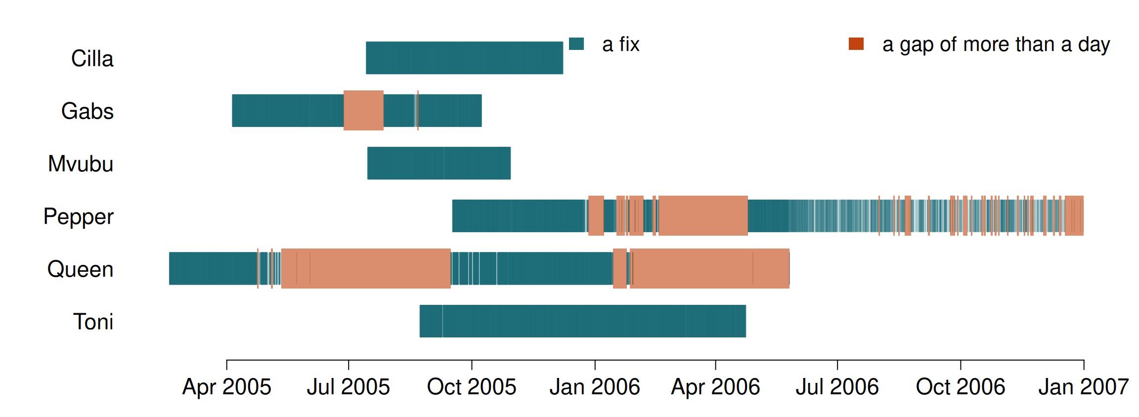
One tick per fix. Queen’s collar went silent for 105 days in mid-2005; Pepper’s schedule frays into gaps through late 2006.

Two ways to hold a trajectory

`adehabitatLT::ltraj`

The classic (Calenge 2006). One data frame per burst, with dist, dt, R2n (squared displacement), abs.angle and rel.angle precomputed.

redisltraj() regularises by interpolating new positions.

`amt::track_xyt`

A tidy tibble. Steps, angles and covariates are computed when you ask.

track_resample() regularises by selecting existing fixes.

The two “regularise” functions do opposite things. One keeps only what you observed; the other manufactures positions you did not observe.

Selecting versus interpolating

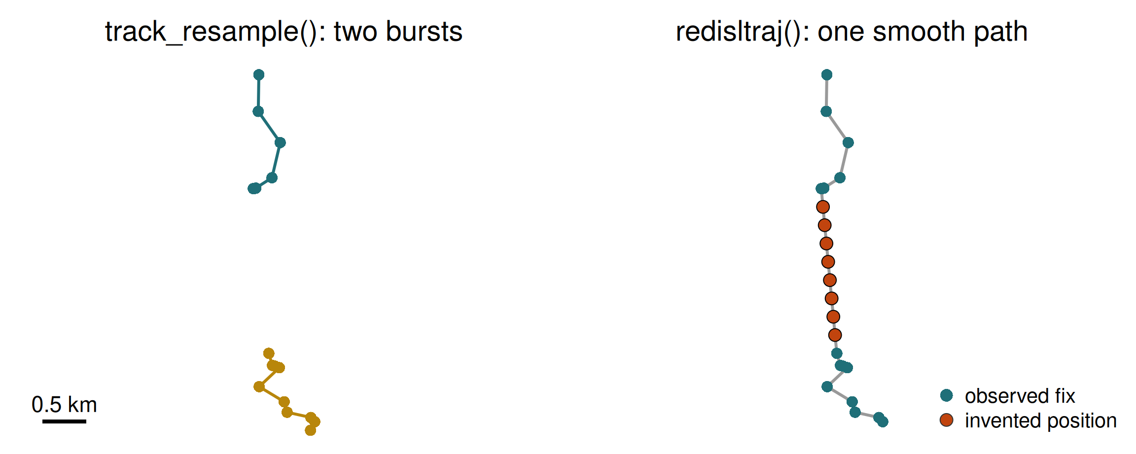
Toni across a 9-hour gap. Selection ends the burst at the gap; interpolation fills it with evenly spaced positions on a straight line the buffalo almost certainly did not walk.

Truncation: the start and the end

After capture — animals often behave abnormally for days (flight, restricted movement). Many studies discard a fixed post-capture window
Before the end — a collar that stops moving may mean a dead animal or a dropped collar, not a resting one
At gaps — a burst ends wherever fixes are missing; steps are never computed across a gap

Decide the truncation rules before you look at the results, write them down, and report how much data they removed.

Resampling and bursts

track_resample() keeps fixes that fall on a regular grid within a tolerance, and labels contiguous runs as bursts.

trk |>
  track_resample(rate = hours(1), tolerance = minutes(10)) |>
  filter_min_n_burst(min_n = 3)

rate — the interval you want
tolerance — how much slack. Too tight and you throw away good data; too loose and “hourly” steps are really 40–80 minutes
A burst breaks wherever a fix is missing. Steps are computed within bursts, never across a gap
min_n = 3 because a turning angle needs three points

The trap: `track_resample()` ignores `group_by()`

# WRONG — one time grid laid across six interleaved animals
trk |> group_by(id) |> track_resample(rate = hours(1))

id	fixes before	grouped (wrong)	per animal (right)
Cilla	3528	2731	3518
Mvubu	2572	166	2544
Queen	4545	1741	4354

# RIGHT — each animal gets its own grid
resample_one <- function(d) {
  track_resample(d, rate = hours(1), tolerance = minutes(10))
}

trk |>
  nest(data = -id) |>
  mutate(data = lapply(data, resample_one)) |>
  unnest(cols = data)

No error, no warning — just 58% of your data gone. Not every function respects dplyr grouping. When a step removes far more than you expected, check the per-group counts before you accept it.

Who tolerates irregular sampling?

Method	Irregular sampling?	Why
MCP, classical KDE	tolerated, with care	uneven sampling over-weights well-sampled periods
Brownian bridge (Session 6)	yes	the bridge’s variance grows with the time between fixes
AKDE / `ctmm` (Session 6)	yes	continuous-time models
SSF (Session 7)	per burst	every step must span the same interval
HMM (Session 8)	no, not directly	discrete time steps; impute a regular grid first (`momentuHMM::crawlWrap`)

Regularity is not a cosmetic property of your data. It decides which methods you are allowed to use.

Quiz

track_resample() interpolates missing locations to give you a regular series. True or false?

True — that is what resampling means
False — it selects existing fixes and discards the rest

amt::track_resample() is a filter, not an interpolator. It walks the track and keeps the fixes that fall close enough to a regular time grid; where no fix is available, the burst simply ends. You never gain observations you did not make.

That is deliberate. Interpolating locations invents data and then feeds the invention into a model as if it were an observation, which biases step-length and turning-angle distributions towards straighter, slower movement.

If you genuinely need locations between fixes, use a model that says so — a continuous-time movement model (ctmm) or a state-space model — which gives you interpolated positions with uncertainty attached.

Quiz

A colleague reports a mean sampling interval of 2.45 hours for a collar programmed to fix hourly. What does that number actually tell you?

The collar was reprogrammed partway through
Almost nothing about the schedule — a few very long gaps have inflated the mean
The fix success rate was about 41%
The animal was inactive, so the collar skipped fixes

The median for this collar is 1 hour — the schedule is intact. The mean is 2.45 h because the distribution has a long tail: one gap of 2,523 hours (105 days) drags it up on its own.

A mean sampling interval is a summary of your collar failures, not of your sampling design. Report the median, the maximum gap, and the number of gaps beyond some threshold.

And no, you cannot read the fix success rate off the mean. Success rate is the proportion of scheduled attempts that returned a location, which you get by dividing each gap by the modal interval and counting the misses.

5 · Attaching the environment

The operation

For every fix, look up the environment there and then.

Static covariates — elevation, slope, distance to river. One raster; extract() and done.
Dynamic covariates — NDVI, temperature, snow. A stack of rasters with timestamps. You must match each fix to the right layer.

A track that spans two years annotated with a single NDVI image is not annotated — it is decorated. If your covariate varies in time and your analysis does not, you have thrown away the mechanism.

Decorated versus annotated

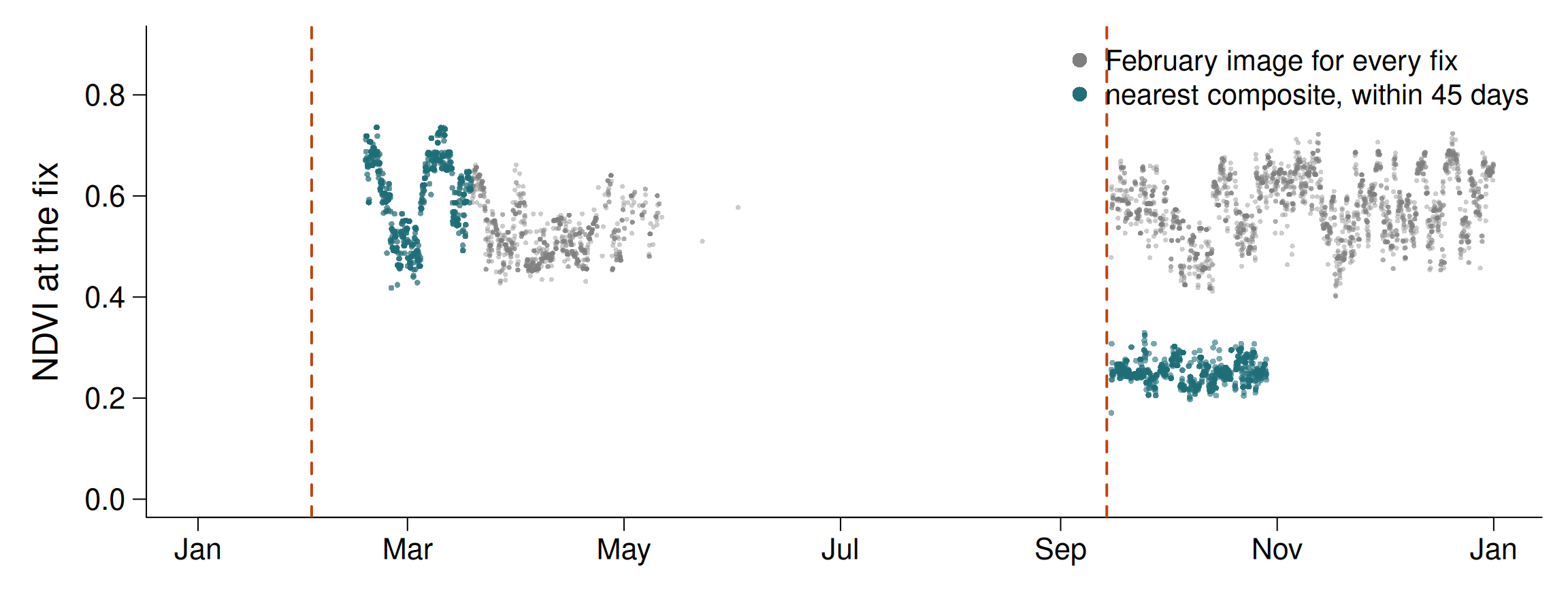
Queen in 2005. One February image says she lived in green vegetation all year. Matched in time, NDVI halves by September — and the months with no composite nearby are honestly blank.

Doing it in time

# Which layer does each fix belong to?
layer_dates <- as.Date(c("2005-01-01", "2005-01-17", ...))

idx <- findInterval(as.Date(trk$t_), layer_dates)

# Extract from the whole stack, then pick the right column per row
vals <- terra::extract(ndvi_stack, vect(trk))[, -1]
trk$ndvi <- vals[cbind(seq_len(nrow(vals)), idx)]

Movebank Env-DATA does this for you, including interpolation in time, for dozens of products. Use it for real projects — but understand what it is doing first, which is what today’s exercise is for.

Quiz

You annotate two years of buffalo fixes with a single dry-season NDVI image and find a strong positive selection for high NDVI. What is the main problem?

NDVI saturates in dense vegetation
The covariate is static while both the animal and the vegetation varied seasonally
The pixel size is too coarse
NDVI cannot be used for savanna

The image describes one moment. Over two years, vegetation in a savanna swings enormously between wet and dry season, and the buffalo’s needs swing with it. By holding NDVI fixed you have conflated “places that were green in that dry season” with “places that are green when the animal was there”.

What you have measured is selection for persistently productive places — which may be interesting, but is not what the model claims.

The result can even be the opposite sign from the time-matched analysis: an animal may select the greenest available patch at every moment while showing no preference for places that are green on average.

Fix: use a time series and match each fix to the contemporaneous layer.

Today’s practical

→ Session 3 practical

Build the same trajectory in adehabitatLT and in amt
Clean it, counting what you remove
Quantify and visualise sampling irregularity
Resample: selection (track_resample) versus interpolation (redisltraj)
Day or night? time_of_day()
Attach NDVI matched to the season of each fix

Recap

A track is a sample of a path; every line between fixes is an assumption
Location error dominates short steps: resting looks random, spikes look like sprints
Clean in order: duplicates → missing → impossible → speed, counting as you go
track_resample() selects; redisltraj() interpolates; track_resample() ignores group_by()
Regularity decides which methods you may use later
Annotate in space and time

Before Session 4

vignette("adehabitatLT", package = "adehabitatLT"), sections on ltraj
Skim Fauchald & Tveraa (2003), Ecology 84:282 — first-passage time

From fixes to trajectories

Today

Where we are going

1 · Positions are not paths

What a GPS track actually is

The step

Steps and turns of a real buffalo

Location error: why you cannot connect the dots

What error looks like

2 · Getting data

Movebank in R

Two object models

move2

amt

Making a track

3 · Cleaning

The four things that are always wrong

Duplicates are not all the same

Speed filtering: useful and dangerous

Quiz

4 · Bursts, gaps and regularity

Why it governs everything

What our buffalo actually look like

Gaps at a glance

Two ways to hold a trajectory

adehabitatLT::ltraj

amt::track_xyt

Selecting versus interpolating

Truncation: the start and the end

Resampling and bursts

The trap: track_resample() ignores group_by()

Who tolerates irregular sampling?

Quiz

Quiz

5 · Attaching the environment

The operation

Decorated versus annotated

Doing it in time

Quiz

Today’s practical

Recap

Before Session 4

`move2`

`amt`

`adehabitatLT::ltraj`

`amt::track_xyt`

The trap: `track_resample()` ignores `group_by()`